
|
|
|
 在 GitHub 上檢視原始碼 在 GitHub 上檢視原始碼
|
|
這個筆記本使用 TensorFlow Core 低階 API,為手寫數字分類建立端對端機器學習工作流程,搭配多層感知器和 MNIST 資料集。請造訪 Core API 總覽,進一步瞭解 TensorFlow Core 及其預期用途。
多層感知器 (MLP) 總覽
多層感知器 (MLP) 是一種前饋神經網路,用於解決多類別分類問題。在建構 MLP 之前,務必先瞭解感知器、層和啟動函數的概念。
多層感知器是由稱為感知器的功能單元組成。感知器的方程式如下
\[Z = \vec{w}⋅\mathrm{X} + b\]
其中
- \(Z\): 感知器輸出
- \(\mathrm{X}\): 特徵矩陣
- \(\vec{w}\): 權重向量
- \(b\): 偏差
當這些感知器堆疊在一起時,會形成稱為密集層的結構,然後可以連接這些結構來建構神經網路。密集層的方程式與感知器的方程式類似,但改用權重矩陣和偏差向量
\[Z = \mathrm{W}⋅\mathrm{X} + \vec{b}\]
其中
- \(Z\): 密集層輸出
- \(\mathrm{X}\): 特徵矩陣
- \(\mathrm{W}\): 權重矩陣
- \(\vec{b}\): 偏差向量
在 MLP 中,多個密集層以某種方式連接,讓某一層的輸出完全連接到下一層的輸入。將非線性啟動函數新增至密集層的輸出,有助於 MLP 分類器學習複雜的決策邊界,並妥善概括未見資料。
設定
匯入 TensorFlow、pandas、Matplotlib 和 seaborn 以開始使用。
# Use seaborn for countplot.pip install -q seaborn
import pandas as pd
import matplotlib
from matplotlib import pyplot as plt
import seaborn as sns
import tempfile
import os
# Preset Matplotlib figure sizes.
matplotlib.rcParams['figure.figsize'] = [9, 6]
import tensorflow as tf
import tensorflow_datasets as tfds
print(tf.__version__)
# Set random seed for reproducible results
tf.random.set_seed(22)
2023-10-04 01:27:29.112043: E tensorflow/compiler/xla/stream_executor/cuda/cuda_dnn.cc:9342] Unable to register cuDNN factory: Attempting to register factory for plugin cuDNN when one has already been registered
2023-10-04 01:27:29.112093: E tensorflow/compiler/xla/stream_executor/cuda/cuda_fft.cc:609] Unable to register cuFFT factory: Attempting to register factory for plugin cuFFT when one has already been registered
2023-10-04 01:27:29.112126: E tensorflow/compiler/xla/stream_executor/cuda/cuda_blas.cc:1518] Unable to register cuBLAS factory: Attempting to register factory for plugin cuBLAS when one has already been registered
2.14.0
載入資料
本教學課程使用 MNIST 資料集,並示範如何建構可分類手寫數字的 MLP 模型。資料集可從 TensorFlow Datasets 取得。
將 MNIST 資料集分割為訓練集、驗證集和測試集。驗證集可用於評估模型在訓練期間的概括能力,讓測試集可做為模型效能的最終不偏估計值。
train_data, val_data, test_data = tfds.load("mnist",
                                            split=['train[10000:]', 'train[0:10000]', 'test'],
                                            batch_size=128, as_supervised=True)
2023-10-04 01:27:32.380134: W tensorflow/core/common_runtime/gpu/gpu_device.cc:2211] Cannot dlopen some GPU libraries. Please make sure the missing libraries mentioned above are installed properly if you would like to use GPU. Follow the guide at https://tensorflow.dev.org.tw/install/gpu for how to download and setup the required libraries for your platform.
Skipping registering GPU devices...
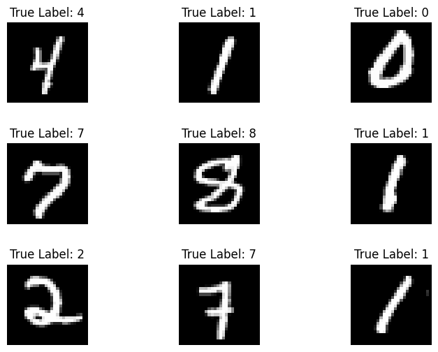
MNIST 資料集包含手寫數字及其對應的真實標籤。在下方視覺化幾個範例。
x_viz, y_viz = tfds.load("mnist", split=['train[:1500]'], batch_size=-1, as_supervised=True)[0]
x_viz = tf.squeeze(x_viz, axis=3)

for i in range(9):
    plt.subplot(3,3,1+i)
    plt.axis('off')
    plt.imshow(x_viz[i], cmap='gray')
    plt.title(f"True Label: {y_viz[i]}")
    plt.subplots_adjust(hspace=.5)
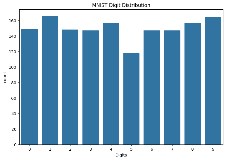
也請檢閱訓練資料中的數字分佈,確認每個類別在資料集中都有充分的代表性。
sns.countplot(x=y_viz.numpy());
plt.xlabel('Digits')
plt.title("MNIST Digit Distribution");
前處理資料
首先,將特徵矩陣重新塑形為二維,方法是將圖片攤平。接著,重新調整資料比例,讓 [0,255] 的像素值符合 [0,1] 的範圍。這個步驟可確保輸入像素具有類似的分佈,並有助於訓練收斂。
def preprocess(x, y):
  # Reshaping the data
  x = tf.reshape(x, shape=[-1, 784])
  # Rescaling the data
  x = x/255
  return x, y

train_data, val_data = train_data.map(preprocess), val_data.map(preprocess)
建構 MLP
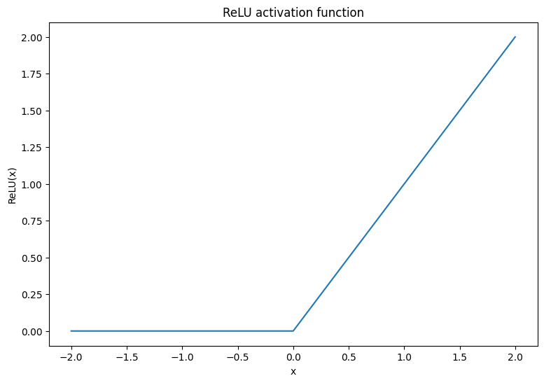
首先,視覺化 ReLU 和 Softmax 啟動函數。這兩個函數分別可在 tf.nn.relu 和 tf.nn.softmax 中取得。ReLU 是非線性啟動函數,如果輸入為正數,則輸出輸入,否則輸出 0
\[\text{ReLU}(X) = max(0, X)\]
x = tf.linspace(-2, 2, 201)
x = tf.cast(x, tf.float32)
plt.plot(x, tf.nn.relu(x));
plt.xlabel('x')
plt.ylabel('ReLU(x)')
plt.title('ReLU activation function');
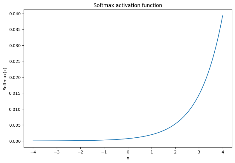
softmax 啟動函數是正規化的指數函數,可將 \(m\) 個實數轉換為具有 \(m\) 個結果/類別的機率分佈。這對於從神經網路的輸出預測類別機率很有用
\[\text{Softmax}(X) = \frac{e^{X} }{\sum_{i=1}^{m}e^{X_i} }\]
x = tf.linspace(-4, 4, 201)
x = tf.cast(x, tf.float32)
plt.plot(x, tf.nn.softmax(x, axis=0));
plt.xlabel('x')
plt.ylabel('Softmax(x)')
plt.title('Softmax activation function');
密集層
為密集層建立類別。依照定義,在 MLP 中,一層的輸出會完全連接到下一層的輸入。因此,密集層的輸入維度可以根據其前一層的輸出維度推斷,不需要在初始化期間預先指定。權重也應妥善初始化,以防止啟動輸出變得過大或過小。最熱門的權重初始化方法之一是 Xavier 配置,其中權重矩陣的每個元素都以下列方式取樣
\[W_{ij} \sim \text{Uniform}(-\frac{\sqrt{6} }{\sqrt{n + m} },\frac{\sqrt{6} }{\sqrt{n + m} })\]
偏差向量可以初始化為零。
def xavier_init(shape):
  # Computes the xavier initialization values for a weight matrix
  in_dim, out_dim = shape
  xavier_lim = tf.sqrt(6.)/tf.sqrt(tf.cast(in_dim + out_dim, tf.float32))
  weight_vals = tf.random.uniform(shape=(in_dim, out_dim),
                                  minval=-xavier_lim, maxval=xavier_lim, seed=22)
  return weight_vals
Xavier 初始化方法也可以透過 tf.keras.initializers.GlorotUniform 實作。
class DenseLayer(tf.Module):

  def __init__(self, out_dim, weight_init=xavier_init, activation=tf.identity):
    # Initialize the dimensions and activation functions
    self.out_dim = out_dim
    self.weight_init = weight_init
    self.activation = activation
    self.built = False

  def __call__(self, x):
    if not self.built:
      # Infer the input dimension based on first call
      self.in_dim = x.shape[1]
      # Initialize the weights and biases
      self.w = tf.Variable(self.weight_init(shape=(self.in_dim, self.out_dim)))
      self.b = tf.Variable(tf.zeros(shape=(self.out_dim,)))
      self.built = True
    # Compute the forward pass
    z = tf.add(tf.matmul(x, self.w), self.b)
    return self.activation(z)
接著,為循序執行各層的 MLP 模型建構類別。請記住,模型變數只有在密集層呼叫的第一個序列之後才能使用,這是因為維度推斷的緣故。
class MLP(tf.Module):

  def __init__(self, layers):
    self.layers = layers

  @tf.function
  def __call__(self, x, preds=False):
    # Execute the model's layers sequentially
    for layer in self.layers:
      x = layer(x)
    return x
使用下列架構初始化 MLP 模型
- 正向傳遞:ReLU(784 x 700) x ReLU(700 x 500) x Softmax(500 x 10)
softmax 啟動函數不需要由 MLP 應用。它會在損失和預測函數中個別計算。
hidden_layer_1_size = 700
hidden_layer_2_size = 500
output_size = 10

mlp_model = MLP([
    DenseLayer(out_dim=hidden_layer_1_size, activation=tf.nn.relu),
    DenseLayer(out_dim=hidden_layer_2_size, activation=tf.nn.relu),
    DenseLayer(out_dim=output_size)])
定義損失函數
交叉熵損失函數是多類別分類問題的絕佳選擇,因為它可以測量資料的負對數概似,依據模型的機率預測。指派給真實類別的機率越高,損失就越低。交叉熵損失的方程式如下
\[L = -\frac{1}{n}\sum_{i=1}^{n}\sum_{i=j}^{n} {y_j}^{[i]}⋅\log(\hat{ {y_j} }^{[i]})\]
其中
- \(\underset{n\times m}{\hat{y} }\): 預測類別分佈的矩陣
- \(\underset{n\times m}{y}\): 真實類別的單熱編碼矩陣
可以使用 tf.nn.sparse_softmax_cross_entropy_with_logits 函數來計算交叉熵損失。這個函數不需要模型的最後一層應用 softmax 啟動函數,也不需要類別標籤採用單熱編碼
def cross_entropy_loss(y_pred, y):
  # Compute cross entropy loss with a sparse operation
  sparse_ce = tf.nn.sparse_softmax_cross_entropy_with_logits(labels=y, logits=y_pred)
  return tf.reduce_mean(sparse_ce)
編寫基本準確度函數,計算訓練期間正確分類的比例。為了從 softmax 輸出產生類別預測,傳回對應於最大類別機率的索引。
def accuracy(y_pred, y):
  # Compute accuracy after extracting class predictions
  class_preds = tf.argmax(tf.nn.softmax(y_pred), axis=1)
  is_equal = tf.equal(y, class_preds)
  return tf.reduce_mean(tf.cast(is_equal, tf.float32))
訓練模型
與標準梯度下降相比,使用最佳化工具可以大幅加快收斂速度。下方實作了 Adam 最佳化工具。請造訪最佳化工具指南,進一步瞭解如何使用 TensorFlow Core 設計自訂最佳化工具。
class Adam:

    def __init__(self, learning_rate=1e-3, beta_1=0.9, beta_2=0.999, ep=1e-7):
      # Initialize optimizer parameters and variable slots
      self.beta_1 = beta_1
      self.beta_2 = beta_2
      self.learning_rate = learning_rate
      self.ep = ep
      self.t = 1.
      self.v_dvar, self.s_dvar = [], []
      self.built = False

    def apply_gradients(self, grads, vars):
      # Initialize variables on the first call
      if not self.built:
        for var in vars:
          v = tf.Variable(tf.zeros(shape=var.shape))
          s = tf.Variable(tf.zeros(shape=var.shape))
          self.v_dvar.append(v)
          self.s_dvar.append(s)
        self.built = True
      # Update the model variables given their gradients
      for i, (d_var, var) in enumerate(zip(grads, vars)):
        self.v_dvar[i].assign(self.beta_1*self.v_dvar[i] + (1-self.beta_1)*d_var)
        self.s_dvar[i].assign(self.beta_2*self.s_dvar[i] + (1-self.beta_2)*tf.square(d_var))
        v_dvar_bc = self.v_dvar[i]/(1-(self.beta_1**self.t))
        s_dvar_bc = self.s_dvar[i]/(1-(self.beta_2**self.t))
        var.assign_sub(self.learning_rate*(v_dvar_bc/(tf.sqrt(s_dvar_bc) + self.ep)))
      self.t += 1.
      return
現在,編寫自訂訓練迴圈,使用迷你批次梯度下降更新 MLP 參數。使用迷你批次進行訓練可同時提供記憶體效率和更快的收斂速度。
def train_step(x_batch, y_batch, loss, acc, model, optimizer):
  # Update the model state given a batch of data
  with tf.GradientTape() as tape:
    y_pred = model(x_batch)
    batch_loss = loss(y_pred, y_batch)
  batch_acc = acc(y_pred, y_batch)
  grads = tape.gradient(batch_loss, model.variables)
  optimizer.apply_gradients(grads, model.variables)
  return batch_loss, batch_acc

def val_step(x_batch, y_batch, loss, acc, model):
  # Evaluate the model on given a batch of validation data
  y_pred = model(x_batch)
  batch_loss = loss(y_pred, y_batch)
  batch_acc = acc(y_pred, y_batch)
  return batch_loss, batch_acc
def train_model(mlp, train_data, val_data, loss, acc, optimizer, epochs):
  # Initialize data structures
  train_losses, train_accs = [], []
  val_losses, val_accs = [], []

  # Format training loop and begin training
  for epoch in range(epochs):
    batch_losses_train, batch_accs_train = [], []
    batch_losses_val, batch_accs_val = [], []

    # Iterate over the training data
    for x_batch, y_batch in train_data:
      # Compute gradients and update the model's parameters
      batch_loss, batch_acc = train_step(x_batch, y_batch, loss, acc, mlp, optimizer)
      # Keep track of batch-level training performance
      batch_losses_train.append(batch_loss)
      batch_accs_train.append(batch_acc)

    # Iterate over the validation data
    for x_batch, y_batch in val_data:
      batch_loss, batch_acc = val_step(x_batch, y_batch, loss, acc, mlp)
      batch_losses_val.append(batch_loss)
      batch_accs_val.append(batch_acc)

    # Keep track of epoch-level model performance
    train_loss, train_acc = tf.reduce_mean(batch_losses_train), tf.reduce_mean(batch_accs_train)
    val_loss, val_acc = tf.reduce_mean(batch_losses_val), tf.reduce_mean(batch_accs_val)
    train_losses.append(train_loss)
    train_accs.append(train_acc)
    val_losses.append(val_loss)
    val_accs.append(val_acc)
    print(f"Epoch: {epoch}")
    print(f"Training loss: {train_loss:.3f}, Training accuracy: {train_acc:.3f}")
    print(f"Validation loss: {val_loss:.3f}, Validation accuracy: {val_acc:.3f}")
  return train_losses, train_accs, val_losses, val_accs
以 128 的批次大小訓練 MLP 模型 10 個週期。硬體加速器 (例如 GPU 或 TPU) 也有助於加快訓練時間。
train_losses, train_accs, val_losses, val_accs = train_model(mlp_model, train_data, val_data,
                                                             loss=cross_entropy_loss, acc=accuracy,
                                                             optimizer=Adam(), epochs=10)
Epoch: 0
Training loss: 0.222, Training accuracy: 0.934
Validation loss: 0.120, Validation accuracy: 0.962
Epoch: 1
Training loss: 0.080, Training accuracy: 0.975
Validation loss: 0.099, Validation accuracy: 0.970
Epoch: 2
Training loss: 0.047, Training accuracy: 0.986
Validation loss: 0.092, Validation accuracy: 0.973
Epoch: 3
Training loss: 0.032, Training accuracy: 0.990
Validation loss: 0.091, Validation accuracy: 0.977
Epoch: 4
Training loss: 0.025, Training accuracy: 0.992
Validation loss: 0.100, Validation accuracy: 0.975
Epoch: 5
Training loss: 0.021, Training accuracy: 0.993
Validation loss: 0.101, Validation accuracy: 0.974
Epoch: 6
Training loss: 0.020, Training accuracy: 0.993
Validation loss: 0.106, Validation accuracy: 0.974
Epoch: 7
Training loss: 0.019, Training accuracy: 0.993
Validation loss: 0.096, Validation accuracy: 0.978
Epoch: 8
Training loss: 0.017, Training accuracy: 0.994
Validation loss: 0.108, Validation accuracy: 0.976
Epoch: 9
Training loss: 0.012, Training accuracy: 0.996
Validation loss: 0.103, Validation accuracy: 0.977
效能評估
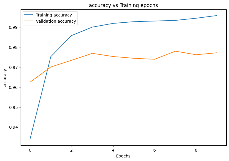
首先,編寫繪圖函數,將模型在訓練期間的損失和準確度視覺化。
def plot_metrics(train_metric, val_metric, metric_type):
  # Visualize metrics vs training Epochs
  plt.figure()
  plt.plot(range(len(train_metric)), train_metric, label = f"Training {metric_type}")
  plt.plot(range(len(val_metric)), val_metric, label = f"Validation {metric_type}")
  plt.xlabel("Epochs")
  plt.ylabel(metric_type)
  plt.legend()
  plt.title(f"{metric_type} vs Training epochs");
plot_metrics(train_losses, val_losses, "cross entropy loss")
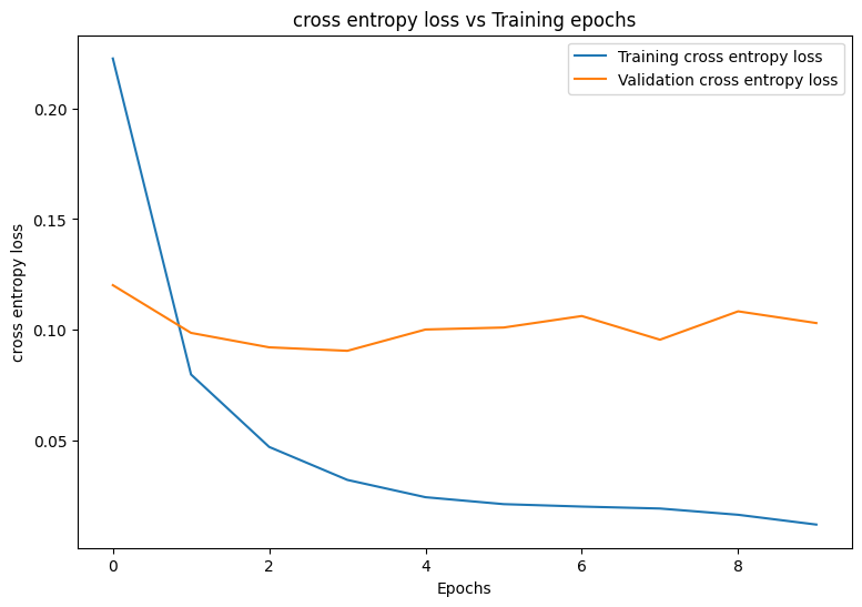
plot_metrics(train_accs, val_accs, "accuracy")
儲存與載入模型
首先,建立匯出模組,接收原始資料並執行下列作業
- 資料前處理
- 機率預測
- 類別預測
class ExportModule(tf.Module):
  def __init__(self, model, preprocess, class_pred):
    # Initialize pre and postprocessing functions
    self.model = model
    self.preprocess = preprocess
    self.class_pred = class_pred

  @tf.function(input_signature=[tf.TensorSpec(shape=[None, None, None, None], dtype=tf.uint8)])
  def __call__(self, x):
    # Run the ExportModule for new data points
    x = self.preprocess(x)
    y = self.model(x)
    y = self.class_pred(y)
    return y
def preprocess_test(x):
  # The export module takes in unprocessed and unlabeled data
  x = tf.reshape(x, shape=[-1, 784])
  x = x/255
  return x

def class_pred_test(y):
  # Generate class predictions from MLP output
  return tf.argmax(tf.nn.softmax(y), axis=1)
現在可以使用 tf.saved_model.save 函數儲存這個匯出模組。
mlp_model_export = ExportModule(model=mlp_model,
                                preprocess=preprocess_test,
                                class_pred=class_pred_test)
models = tempfile.mkdtemp()
save_path = os.path.join(models, 'mlp_model_export')
tf.saved_model.save(mlp_model_export, save_path)
INFO:tensorflow:Assets written to: /tmpfs/tmp/tmphtbcg1os/mlp_model_export/assets
INFO:tensorflow:Assets written to: /tmpfs/tmp/tmphtbcg1os/mlp_model_export/assets
使用 tf.saved_model.load 載入已儲存的模型,並檢查其在未見測試資料上的效能。
mlp_loaded = tf.saved_model.load(save_path)
def accuracy_score(y_pred, y):
  # Generic accuracy function
  is_equal = tf.equal(y_pred, y)
  return tf.reduce_mean(tf.cast(is_equal, tf.float32))

x_test, y_test = tfds.load("mnist", split=['test'], batch_size=-1, as_supervised=True)[0]
test_classes = mlp_loaded(x_test)
test_acc = accuracy_score(test_classes, y_test)
print(f"Test Accuracy: {test_acc:.3f}")
Test Accuracy: 0.979
模型在分類訓練資料集中的手寫數字方面表現出色,並且也能妥善概括未見資料。現在,檢查模型的類別準確度,確保每個數字都有良好的效能。
print("Accuracy breakdown by digit:")
print("---------------------------")
label_accs = {}
for label in range(10):
  label_ind = (y_test == label)
  # extract predictions for specific true label
  pred_label = test_classes[label_ind]
  labels = y_test[label_ind]
  # compute class-wise accuracy
  label_accs[accuracy_score(pred_label, labels).numpy()] = label
for key in sorted(label_accs):
  print(f"Digit {label_accs[key]}: {key:.3f}")
Accuracy breakdown by digit:
---------------------------
Digit 4: 0.960
Digit 7: 0.967
Digit 3: 0.969
Digit 6: 0.973
Digit 8: 0.977
Digit 9: 0.984
Digit 0: 0.989
Digit 2: 0.990
Digit 5: 0.991
Digit 1: 0.993
模型在某些數字上的表現似乎比其他數字吃力一些,這在許多多類別分類問題中相當常見。最後一個練習是繪製模型預測的混淆矩陣及其對應的真實標籤,以收集更多類別層級的深入分析。Sklearn 和 seaborn 具有產生混淆矩陣並將其視覺化的函數。
import sklearn.metrics as sk_metrics

def show_confusion_matrix(test_labels, test_classes):
  # Compute confusion matrix and normalize
  plt.figure(figsize=(10,10))
  confusion = sk_metrics.confusion_matrix(test_labels.numpy(),
                                          test_classes.numpy())
  confusion_normalized = confusion / confusion.sum(axis=1, keepdims=True)
  axis_labels = range(10)
  ax = sns.heatmap(
      confusion_normalized, xticklabels=axis_labels, yticklabels=axis_labels,
      cmap='Blues', annot=True, fmt='.4f', square=True)
  plt.title("Confusion matrix")
  plt.ylabel("True label")
  plt.xlabel("Predicted label")

show_confusion_matrix(y_test, test_classes)
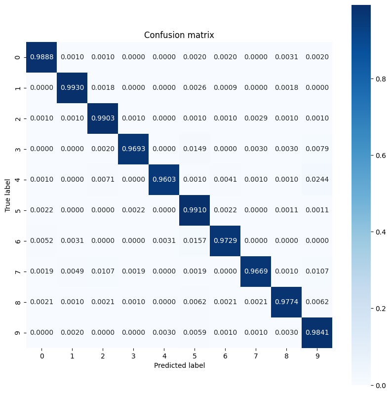
類別層級的深入分析有助於找出錯誤分類的原因,並在未來的訓練週期中提升模型效能。
結論
這個筆記本介紹了一些使用 MLP 處理多類別分類問題的技巧。以下是一些可能有幫助的訣竅
- 可以使用 TensorFlow Core API 建構具有高度可配置性的機器學習工作流程
- 初始化配置有助於防止模型參數在訓練期間消失或爆炸。
- 過度擬合是神經網路的另一個常見問題,雖然它不是本教學課程的問題。請造訪過度擬合與欠擬合教學課程,以取得更多相關協助。
如需使用 TensorFlow Core API 的更多範例,請查看指南。如果您想進一步瞭解如何載入和準備資料,請參閱關於圖片資料載入或 CSV 資料載入的教學課程。