
|
|
|
 在 GitHub 上檢視原始碼 在 GitHub 上檢視原始碼
|
|
簡介
這個筆記本使用 TensorFlow Core 低階 API 和 DTensor 來示範資料平行分散式訓練範例。請造訪 Core API 總覽,進一步瞭解 TensorFlow Core 及其預期的使用案例。請參閱 DTensor 總覽 指南和 使用 DTensor 進行分散式訓練 教學課程,進一步瞭解 DTensor。
這個範例使用 多層感知器 教學課程中顯示的相同模型和最佳化工具。請先參閱這個教學課程,熟悉如何使用 Core API 編寫端對端機器學習工作流程。
使用 DTensor 進行資料平行訓練的總覽
在建構支援分散式的 MLP 之前,請先花一點時間探索 DTensor 用於資料平行訓練的基本原理。
DTensor 可讓您跨裝置執行分散式訓練,以提高效率、可靠性和擴充性。DTensor 會透過稱為單一程式多資料 (SPMD) 擴充的程序,根據分shard 指令分配程式和張量。感知 DTensor 的層的變數會建立為 dtensor.DVariable,而感知 DTensor 的層物件的建構函式除了通常的層參數之外,還會採用額外的 Layout 輸入。
資料平行訓練的主要概念如下
- 模型變數會在每個 N 個裝置上複製。
- 全域批次會分割成 N 個每個複本批次。
- 每個複本批次都會在複本裝置上進行訓練。
- 梯度會在權重升級資料在所有複本上集體執行之前縮減。
- 資料平行訓練提供近乎線性的速度,與裝置數量成正比
設定
DTensor 是 TensorFlow 2.9.0 版本的一部分。
#!pip install --quiet --upgrade --pre tensorflow
import matplotlib
from matplotlib import pyplot as plt
# Preset Matplotlib figure sizes.
matplotlib.rcParams['figure.figsize'] = [9, 6]
import tensorflow as tf
import tensorflow_datasets as tfds
from tensorflow.experimental import dtensor
print(tf.__version__)
# Set random seed for reproducible results
tf.random.set_seed(22)
2023-10-04 01:30:56.221874: E tensorflow/compiler/xla/stream_executor/cuda/cuda_dnn.cc:9342] Unable to register cuDNN factory: Attempting to register factory for plugin cuDNN when one has already been registered
2023-10-04 01:30:56.221918: E tensorflow/compiler/xla/stream_executor/cuda/cuda_fft.cc:609] Unable to register cuFFT factory: Attempting to register factory for plugin cuFFT when one has already been registered
2023-10-04 01:30:56.221966: E tensorflow/compiler/xla/stream_executor/cuda/cuda_blas.cc:1518] Unable to register cuBLAS factory: Attempting to register factory for plugin cuBLAS when one has already been registered
2.14.0
為這個實驗設定 8 個虛擬 CPU。DTensor 也可以與 GPU 或 TPU 裝置搭配使用。由於這個筆記本使用虛擬裝置,因此分散式訓練所獲得的加速效果並不顯著。
def configure_virtual_cpus(ncpu):
  phy_devices = tf.config.list_physical_devices('CPU')
  tf.config.set_logical_device_configuration(phy_devices[0], [
        tf.config.LogicalDeviceConfiguration(),
    ] * ncpu)

configure_virtual_cpus(8)

DEVICES = [f'CPU:{i}' for i in range(8)]
devices = tf.config.list_logical_devices('CPU')
device_names = [d.name for d in devices]
device_names
2023-10-04 01:30:59.029163: W tensorflow/core/common_runtime/gpu/gpu_device.cc:2211] Cannot dlopen some GPU libraries. Please make sure the missing libraries mentioned above are installed properly if you would like to use GPU. Follow the guide at https://tensorflow.dev.org.tw/install/gpu for how to download and setup the required libraries for your platform.
Skipping registering GPU devices...
['/device:CPU:0',
 '/device:CPU:1',
 '/device:CPU:2',
 '/device:CPU:3',
 '/device:CPU:4',
 '/device:CPU:5',
 '/device:CPU:6',
 '/device:CPU:7']
MNIST 資料集
這個資料集可從 TensorFlow Datasets 取得。將資料分割成訓練集和測試集。僅使用 5000 個範例進行訓練和測試,以節省時間。
train_data, test_data = tfds.load("mnist", split=['train[:5000]', 'test[:5000]'], batch_size=128, as_supervised=True)
預先處理資料
預先處理資料的方式是將其重新塑形為二維,並將其重新調整大小以符合單位區間 [0,1]。
def preprocess(x, y):
  # Reshaping the data
  x = tf.reshape(x, shape=[-1, 784])
  # Rescaling the data
  x = x/255
  return x, y

train_data, test_data = train_data.map(preprocess), test_data.map(preprocess)
建構 MLP
使用感知 DTensor 的層建構 MLP 模型。
密集層
首先建立支援 DTensor 的密集層模組。dtensor.call_with_layout 函式可用於呼叫函式,該函式會接收 DTensor 輸入並產生 DTensor 輸出。這適用於使用 TensorFlow 支援的函式初始化 DTensor 變數 dtensor.DVariable。
class DenseLayer(tf.Module):

  def __init__(self, in_dim, out_dim, weight_layout, activation=tf.identity):
    super().__init__()
    # Initialize dimensions and the activation function
    self.in_dim, self.out_dim = in_dim, out_dim
    self.activation = activation

    # Initialize the DTensor weights using the Xavier scheme
    uniform_initializer = tf.function(tf.random.stateless_uniform)
    xavier_lim = tf.sqrt(6.)/tf.sqrt(tf.cast(self.in_dim + self.out_dim, tf.float32))
    self.w = dtensor.DVariable(
      dtensor.call_with_layout(
          uniform_initializer, weight_layout,
          shape=(self.in_dim, self.out_dim), seed=(22, 23),
          minval=-xavier_lim, maxval=xavier_lim))

    # Initialize the bias with the zeros
    bias_layout = weight_layout.delete([0])
    self.b = dtensor.DVariable(
      dtensor.call_with_layout(tf.zeros, bias_layout, shape=[out_dim]))

  def __call__(self, x):
    # Compute the forward pass
    z = tf.add(tf.matmul(x, self.w), self.b)
    return self.activation(z)
MLP 循序模型
現在建立循序執行密集層的 MLP 模組。
class MLP(tf.Module):

  def __init__(self, layers):
    self.layers = layers

  def __call__(self, x, preds=False):
    # Execute the model's layers sequentially
    for layer in self.layers:
      x = layer(x)
    return x
使用 DTensor 執行「資料平行」訓練相當於 tf.distribute.MirroredStrategy。若要執行此操作,每個裝置都會在資料批次的 shard 上執行相同的模型。因此,您需要下列項目
- 具有單一
"batch"維度的dtensor.Mesh - 所有權重的
dtensor.Layout,在網格中複製權重 (每個軸使用dtensor.UNSHARDED) - 資料的
dtensor.Layout,將批次維度分割到網格中
建立包含單一批次維度的 DTensor 網格,其中每個裝置都會成為接收來自全域批次的 shard 的複本。使用這個網格來例項化具有下列架構的 MLP 模式
前向傳遞:ReLU(784 x 700) x ReLU(700 x 500) x Softmax(500 x 10)
mesh = dtensor.create_mesh([("batch", 8)], devices=DEVICES)
weight_layout = dtensor.Layout([dtensor.UNSHARDED, dtensor.UNSHARDED], mesh)

input_size = 784
hidden_layer_1_size = 700
hidden_layer_2_size = 500
hidden_layer_2_size = 10

mlp_model = MLP([
    DenseLayer(in_dim=input_size, out_dim=hidden_layer_1_size,
               weight_layout=weight_layout,
               activation=tf.nn.relu),
    DenseLayer(in_dim=hidden_layer_1_size , out_dim=hidden_layer_2_size,
               weight_layout=weight_layout,
               activation=tf.nn.relu),
    DenseLayer(in_dim=hidden_layer_2_size, out_dim=hidden_layer_2_size,
               weight_layout=weight_layout)])
訓練指標
將交叉熵損失函數和準確度指標用於訓練。
def cross_entropy_loss(y_pred, y):
  # Compute cross entropy loss with a sparse operation
  sparse_ce = tf.nn.sparse_softmax_cross_entropy_with_logits(labels=y, logits=y_pred)
  return tf.reduce_mean(sparse_ce)

def accuracy(y_pred, y):
  # Compute accuracy after extracting class predictions
  class_preds = tf.argmax(y_pred, axis=1)
  is_equal = tf.equal(y, class_preds)
  return tf.reduce_mean(tf.cast(is_equal, tf.float32))
最佳化工具
與標準梯度下降相比,使用最佳化工具可以顯著加快收斂速度。Adam 最佳化工具實作如下,並已設定為與 DTensor 相容。若要將 Keras 最佳化工具與 DTensor 搭配使用,請參閱實驗性 tf.keras.dtensor.experimental.optimizers 模組。
class Adam(tf.Module):

    def __init__(self, model_vars, learning_rate=1e-3, beta_1=0.9, beta_2=0.999, ep=1e-7):
      # Initialize optimizer parameters and variable slots
      self.model_vars = model_vars
      self.beta_1 = beta_1
      self.beta_2 = beta_2
      self.learning_rate = learning_rate
      self.ep = ep
      self.t = 1.
      self.v_dvar, self.s_dvar = [], []
      # Initialize optimizer variable slots
      for var in model_vars:
        v = dtensor.DVariable(dtensor.call_with_layout(tf.zeros, var.layout, shape=var.shape))
        s = dtensor.DVariable(dtensor.call_with_layout(tf.zeros, var.layout, shape=var.shape))
        self.v_dvar.append(v)
        self.s_dvar.append(s)

    def apply_gradients(self, grads):
      # Update the model variables given their gradients
      for i, (d_var, var) in enumerate(zip(grads, self.model_vars)):
        self.v_dvar[i].assign(self.beta_1*self.v_dvar[i] + (1-self.beta_1)*d_var)
        self.s_dvar[i].assign(self.beta_2*self.s_dvar[i] + (1-self.beta_2)*tf.square(d_var))
        v_dvar_bc = self.v_dvar[i]/(1-(self.beta_1**self.t))
        s_dvar_bc = self.s_dvar[i]/(1-(self.beta_2**self.t))
        var.assign_sub(self.learning_rate*(v_dvar_bc/(tf.sqrt(s_dvar_bc) + self.ep)))
      self.t += 1.
      return
資料封裝
首先編寫協助程式函式,用於將資料傳輸到裝置。這個函式應使用 dtensor.pack 來傳送 (且僅傳送) 全域批次的 shard,該 shard 適用於支援複本的裝置。為簡化起見,假設為單一用戶端應用程式。
接下來,編寫一個函式,使用這個協助程式函式將訓練資料批次封裝到沿著批次 (第一個) 軸分shard 的 DTensor 中。這可確保 DTensor 將訓練資料平均分配到「批次」網格維度。請注意,在 DTensor 中,批次大小一律是指全域批次大小;因此,應選擇批次大小,使其可被批次網格維度的大小均勻分割。簡化 tf.data 整合的其他 DTensor API 已在規劃中,敬請期待。
def repack_local_tensor(x, layout):
  # Repacks a local Tensor-like to a DTensor with layout
  # This function assumes a single-client application
  x = tf.convert_to_tensor(x)
  sharded_dims = []

  # For every sharded dimension, use tf.split to split the along the dimension.
  # The result is a nested list of split-tensors in queue[0].
  queue = [x]
  for axis, dim in enumerate(layout.sharding_specs):
    if dim == dtensor.UNSHARDED:
      continue
    num_splits = layout.shape[axis]
    queue = tf.nest.map_structure(lambda x: tf.split(x, num_splits, axis=axis), queue)
    sharded_dims.append(dim)

  # Now you can build the list of component tensors by looking up the location in
  # the nested list of split-tensors created in queue[0].
  components = []
  for locations in layout.mesh.local_device_locations():
    t = queue[0]
    for dim in sharded_dims:
      split_index = locations[dim]  # Only valid on single-client mesh.
      t = t[split_index]
    components.append(t)

  return dtensor.pack(components, layout)

def repack_batch(x, y, mesh):
  # Pack training data batches into DTensors along the batch axis
  x = repack_local_tensor(x, layout=dtensor.Layout(['batch', dtensor.UNSHARDED], mesh))
  y = repack_local_tensor(y, layout=dtensor.Layout(['batch'], mesh))
  return x, y
訓練
編寫可追蹤的函式,該函式會針對指定的資料批次執行單一訓練步驟。這個函式不需要任何特殊的 DTensor 註解。也編寫一個函式,執行測試步驟並傳回適當的效能指標。
@tf.function
def train_step(model, x_batch, y_batch, loss, metric, optimizer):
  # Execute a single training step
  with tf.GradientTape() as tape:
    y_pred = model(x_batch)
    batch_loss = loss(y_pred, y_batch)
  # Compute gradients and update the model's parameters
  grads = tape.gradient(batch_loss, model.trainable_variables)
  optimizer.apply_gradients(grads)
  # Return batch loss and accuracy
  batch_acc = metric(y_pred, y_batch)
  return batch_loss, batch_acc

@tf.function
def test_step(model, x_batch, y_batch, loss, metric):
  # Execute a single testing step
  y_pred = model(x_batch)
  batch_loss = loss(y_pred, y_batch)
  batch_acc = metric(y_pred, y_batch)
  return batch_loss, batch_acc
現在,以 128 的批次大小訓練 MLP 模型 3 個 epoch。
# Initialize the training loop parameters and structures
epochs = 3
batch_size = 128
train_losses, test_losses = [], []
train_accs, test_accs = [], []
optimizer = Adam(mlp_model.trainable_variables)

# Format training loop
for epoch in range(epochs):
  batch_losses_train, batch_accs_train = [], []
  batch_losses_test, batch_accs_test = [], []

  # Iterate through training data
  for x_batch, y_batch in train_data:
    x_batch, y_batch = repack_batch(x_batch, y_batch, mesh)
    batch_loss, batch_acc = train_step(mlp_model, x_batch, y_batch, cross_entropy_loss, accuracy, optimizer)
   # Keep track of batch-level training performance
    batch_losses_train.append(batch_loss)
    batch_accs_train.append(batch_acc)

  # Iterate through testing data
  for x_batch, y_batch in test_data:
    x_batch, y_batch = repack_batch(x_batch, y_batch, mesh)
    batch_loss, batch_acc = test_step(mlp_model, x_batch, y_batch, cross_entropy_loss, accuracy)
    # Keep track of batch-level testing
    batch_losses_test.append(batch_loss)
    batch_accs_test.append(batch_acc)

# Keep track of epoch-level model performance
  train_loss, train_acc = tf.reduce_mean(batch_losses_train), tf.reduce_mean(batch_accs_train)
  test_loss, test_acc = tf.reduce_mean(batch_losses_test), tf.reduce_mean(batch_accs_test)
  train_losses.append(train_loss)
  train_accs.append(train_acc)
  test_losses.append(test_loss)
  test_accs.append(test_acc)
  print(f"Epoch: {epoch}")
  print(f"Training loss: {train_loss.numpy():.3f}, Training accuracy: {train_acc.numpy():.3f}")
  print(f"Testing loss: {test_loss.numpy():.3f}, Testing accuracy: {test_acc.numpy():.3f}")
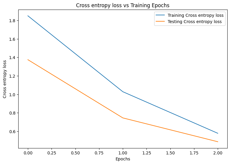
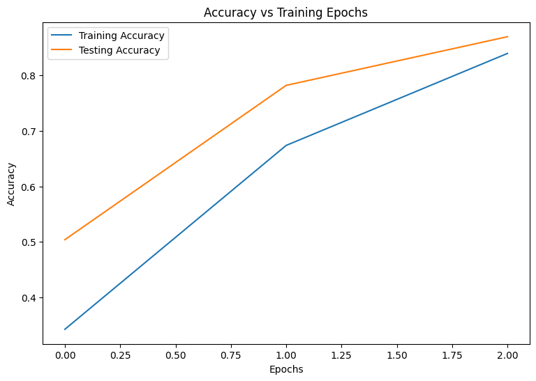
Epoch: 0
Training loss: 1.850, Training accuracy: 0.343
Testing loss: 1.375, Testing accuracy: 0.504
Epoch: 1
Training loss: 1.028, Training accuracy: 0.674
Testing loss: 0.744, Testing accuracy: 0.782
Epoch: 2
Training loss: 0.578, Training accuracy: 0.839
Testing loss: 0.486, Testing accuracy: 0.869
效能評估
首先編寫繪圖函式,將模型在訓練期間的損失和準確度視覺化。
def plot_metrics(train_metric, test_metric, metric_type):
  # Visualize metrics vs training Epochs
  plt.figure()
  plt.plot(range(len(train_metric)), train_metric, label = f"Training {metric_type}")
  plt.plot(range(len(test_metric)), test_metric, label = f"Testing {metric_type}")
  plt.xlabel("Epochs")
  plt.ylabel(metric_type)
  plt.legend()
  plt.title(f"{metric_type} vs Training Epochs");
plot_metrics(train_losses, test_losses, "Cross entropy loss")
plot_metrics(train_accs, test_accs, "Accuracy")
儲存模型
tf.saved_model 和 DTensor 的整合仍在開發中。截至 TensorFlow 2.9.0,tf.saved_model 僅接受具有完全複製變數的 DTensor 模型。作為替代方案,您可以透過重新載入檢查點,將 DTensor 模型轉換為完全複製的模型。但是,在儲存模型之後,所有 DTensor 註解都會遺失,且儲存的簽章只能與一般張量搭配使用。這個教學課程將在整合完成後更新,以展示整合。
結論
這個筆記本概述了使用 DTensor 和 TensorFlow Core API 進行分散式訓練。以下是一些可能有幫助的訣竅
- TensorFlow Core API 可用於建構高度可設定的機器學習工作流程,並支援分散式訓練。
- DTensor 概念 指南和 使用 DTensor 進行分散式訓練 教學課程包含有關 DTensor 及其整合的最新資訊。
如需使用 TensorFlow Core API 的更多範例,請查看指南。如果您想進一步瞭解如何載入和準備資料,請參閱關於 圖片資料載入 或 CSV 資料載入 的教學課程。