使用 3D 卷積神經網路進行影片分類

在 TensorFlow.org 上檢視

在 Google Colab 中執行

在 GitHub 上檢視原始碼

下載筆記本

本教學課程示範如何使用 UCF101 動作辨識資料集，訓練用於影片分類的 3D 卷積神經網路 (CNN)。3D CNN 使用三維篩選器執行卷積。核心能夠在三個方向上滑動，而 2D CNN 則只能在兩個維度上滑動。此模型是以 D. Tran 等人發表的著作 A Closer Look at Spatiotemporal Convolutions for Action Recognition (2017) 為基礎。在本教學課程中，您將：

• 建立輸入管線
• 使用 Keras Functional API 建立具有殘差連線的 3D 卷積神經網路模型
• 訓練模型
• 評估及測試模型

本影片分類教學課程是 TensorFlow 影片教學課程系列的第二部分。以下是其他三個教學課程：

• 載入影片資料：本教學課程說明本文件中使用的許多程式碼。
• 用於串流動作辨識的 MoViNet：熟悉 TF Hub 上提供的 MoViNet 模型。
• 使用 MoViNet 進行影片分類遷移學習：本教學課程說明如何將在不同資料集上訓練的預先訓練影片分類模型與 UCF-101 資料集搭配使用。

設定

首先安裝並匯入一些必要的程式庫，包括：remotezip (用於檢查 ZIP 檔案的內容)、tqdm (用於使用進度列)、OpenCV (用於處理影片檔案)、einops (用於執行更複雜的張量運算)，以及 tensorflow_docs (用於在 Jupyter 筆記本中嵌入資料)。

pip install remotezip tqdm opencv-python einops
pip install -U tensorflow keras

import tqdm
import random
import pathlib
import itertools
import collections

import cv2
import einops
import numpy as np
import remotezip as rz
import seaborn as sns
import matplotlib.pyplot as plt

import tensorflow as tf
import keras
from keras import layers

2024-07-13 04:45:46.026708: E external/local_xla/xla/stream_executor/cuda/cuda_fft.cc:485] Unable to register cuFFT factory: Attempting to register factory for plugin cuFFT when one has already been registered
2024-07-13 04:45:46.048378: E external/local_xla/xla/stream_executor/cuda/cuda_dnn.cc:8454] Unable to register cuDNN factory: Attempting to register factory for plugin cuDNN when one has already been registered
2024-07-13 04:45:46.054995: E external/local_xla/xla/stream_executor/cuda/cuda_blas.cc:1452] Unable to register cuBLAS factory: Attempting to register factory for plugin cuBLAS when one has already been registered

載入與預先處理影片資料

下方的隱藏儲存格定義了輔助函式，用於從 UCF-101 資料集下載部分資料，並將其載入 tf.data.Dataset。您可以在載入影片資料教學課程中進一步瞭解特定的預先處理步驟，該教學課程會更詳細地逐步說明此程式碼。

隱藏區塊結尾的 FrameGenerator 類別是此處最重要的公用程式。它會建立可迭代的物件，可將資料饋送到 TensorFlow 資料管線中。具體來說，此類別包含 Python 產生器，可載入影片影格及其編碼標籤。產生器 (__call__) 函式會產生由 frames_from_video_file 產生的影格陣列，以及與影格集相關聯的標籤的單熱編碼向量。

def list_files_per_class(zip_url):
  """
    List the files in each class of the dataset given the zip URL.

    Args:
      zip_url: URL from which the files can be unzipped. 

    Return:
      files: List of files in each of the classes.
  """
  files = []
  with rz.RemoteZip(URL) as zip:
    for zip_info in zip.infolist():
      files.append(zip_info.filename)
  return files

def get_class(fname):
  """
    Retrieve the name of the class given a filename.

    Args:
      fname: Name of the file in the UCF101 dataset.

    Return:
      Class that the file belongs to.
  """
  return fname.split('_')[-3]

def get_files_per_class(files):
  """
    Retrieve the files that belong to each class. 

    Args:
      files: List of files in the dataset.

    Return:
      Dictionary of class names (key) and files (values).
  """
  files_for_class = collections.defaultdict(list)
  for fname in files:
    class_name = get_class(fname)
    files_for_class[class_name].append(fname)
  return files_for_class

def download_from_zip(zip_url, to_dir, file_names):
  """
    Download the contents of the zip file from the zip URL.

    Args:
      zip_url: Zip URL containing data.
      to_dir: Directory to download data to.
      file_names: Names of files to download.
  """
  with rz.RemoteZip(zip_url) as zip:
    for fn in tqdm.tqdm(file_names):
      class_name = get_class(fn)
      zip.extract(fn, str(to_dir / class_name))
      unzipped_file = to_dir / class_name / fn

      fn = pathlib.Path(fn).parts[-1]
      output_file = to_dir / class_name / fn
      unzipped_file.rename(output_file,)

def split_class_lists(files_for_class, count):
  """
    Returns the list of files belonging to a subset of data as well as the remainder of
    files that need to be downloaded.

    Args:
      files_for_class: Files belonging to a particular class of data.
      count: Number of files to download.

    Return:
      split_files: Files belonging to the subset of data.
      remainder: Dictionary of the remainder of files that need to be downloaded.
  """
  split_files = []
  remainder = {}
  for cls in files_for_class:
    split_files.extend(files_for_class[cls][:count])
    remainder[cls] = files_for_class[cls][count:]
  return split_files, remainder

def download_ufc_101_subset(zip_url, num_classes, splits, download_dir):
  """
    Download a subset of the UFC101 dataset and split them into various parts, such as
    training, validation, and test. 

    Args:
      zip_url: Zip URL containing data.
      num_classes: Number of labels.
      splits: Dictionary specifying the training, validation, test, etc. (key) division of data 
              (value is number of files per split).
      download_dir: Directory to download data to.

    Return:
      dir: Posix path of the resulting directories containing the splits of data.
  """
  files = list_files_per_class(zip_url)
  for f in files:
    tokens = f.split('/')
    if len(tokens) <= 2:
      files.remove(f) # Remove that item from the list if it does not have a filename

  files_for_class = get_files_per_class(files)

  classes = list(files_for_class.keys())[:num_classes]

  for cls in classes:
    new_files_for_class = files_for_class[cls]
    random.shuffle(new_files_for_class)
    files_for_class[cls] = new_files_for_class

  # Only use the number of classes you want in the dictionary
  files_for_class = {x: files_for_class[x] for x in list(files_for_class)[:num_classes]}

  dirs = {}
  for split_name, split_count in splits.items():
    print(split_name, ":")
    split_dir = download_dir / split_name
    split_files, files_for_class = split_class_lists(files_for_class, split_count)
    download_from_zip(zip_url, split_dir, split_files)
    dirs[split_name] = split_dir

  return dirs

def format_frames(frame, output_size):
  """
    Pad and resize an image from a video.

    Args:
      frame: Image that needs to resized and padded. 
      output_size: Pixel size of the output frame image.

    Return:
      Formatted frame with padding of specified output size.
  """
  frame = tf.image.convert_image_dtype(frame, tf.float32)
  frame = tf.image.resize_with_pad(frame, *output_size)
  return frame

def frames_from_video_file(video_path, n_frames, output_size = (224,224), frame_step = 15):
  """
    Creates frames from each video file present for each category.

    Args:
      video_path: File path to the video.
      n_frames: Number of frames to be created per video file.
      output_size: Pixel size of the output frame image.

    Return:
      An NumPy array of frames in the shape of (n_frames, height, width, channels).
  """
  # Read each video frame by frame
  result = []
  src = cv2.VideoCapture(str(video_path))  

  video_length = src.get(cv2.CAP_PROP_FRAME_COUNT)

  need_length = 1 + (n_frames - 1) * frame_step

  if need_length > video_length:
    start = 0
  else:
    max_start = video_length - need_length
    start = random.randint(0, max_start + 1)

  src.set(cv2.CAP_PROP_POS_FRAMES, start)
  # ret is a boolean indicating whether read was successful, frame is the image itself
  ret, frame = src.read()
  result.append(format_frames(frame, output_size))

  for _ in range(n_frames - 1):
    for _ in range(frame_step):
      ret, frame = src.read()
    if ret:
      frame = format_frames(frame, output_size)
      result.append(frame)
    else:
      result.append(np.zeros_like(result[0]))
  src.release()
  result = np.array(result)[..., [2, 1, 0]]

  return result

class FrameGenerator:
  def __init__(self, path, n_frames, training = False):
    """ Returns a set of frames with their associated label. 

      Args:
        path: Video file paths.
        n_frames: Number of frames. 
        training: Boolean to determine if training dataset is being created.
    """
    self.path = path
    self.n_frames = n_frames
    self.training = training
    self.class_names = sorted(set(p.name for p in self.path.iterdir() if p.is_dir()))
    self.class_ids_for_name = dict((name, idx) for idx, name in enumerate(self.class_names))

  def get_files_and_class_names(self):
    video_paths = list(self.path.glob('*/*.avi'))
    classes = [p.parent.name for p in video_paths] 
    return video_paths, classes

  def __call__(self):
    video_paths, classes = self.get_files_and_class_names()

    pairs = list(zip(video_paths, classes))

    if self.training:
      random.shuffle(pairs)

    for path, name in pairs:
      video_frames = frames_from_video_file(path, self.n_frames) 
      label = self.class_ids_for_name[name] # Encode labels
      yield video_frames, label

URL = 'https://storage.googleapis.com/thumos14_files/UCF101_videos.zip'
download_dir = pathlib.Path('./UCF101_subset/')
subset_paths = download_ufc_101_subset(URL, 
                        num_classes = 10, 
                        splits = {"train": 30, "val": 10, "test": 10},
                        download_dir = download_dir)

train :
100%|██████████| 300/300 [00:25<00:00, 11.66it/s]
val :
100%|██████████| 100/100 [00:11<00:00,  8.86it/s]
test :
100%|██████████| 100/100 [00:07<00:00, 12.55it/s]

建立訓練、驗證和測試集 (train_ds、val_ds 和 test_ds)。

n_frames = 10
batch_size = 8

output_signature = (tf.TensorSpec(shape = (None, None, None, 3), dtype = tf.float32),
                    tf.TensorSpec(shape = (), dtype = tf.int16))

train_ds = tf.data.Dataset.from_generator(FrameGenerator(subset_paths['train'], n_frames, training=True),
                                          output_signature = output_signature)


# Batch the data
train_ds = train_ds.batch(batch_size)

val_ds = tf.data.Dataset.from_generator(FrameGenerator(subset_paths['val'], n_frames),
                                        output_signature = output_signature)
val_ds = val_ds.batch(batch_size)

test_ds = tf.data.Dataset.from_generator(FrameGenerator(subset_paths['test'], n_frames),
                                         output_signature = output_signature)

test_ds = test_ds.batch(batch_size)

WARNING: All log messages before absl::InitializeLog() is called are written to STDERR
I0000 00:00:1720845994.489541  108593 cuda_executor.cc:1015] successful NUMA node read from SysFS had negative value (-1), but there must be at least one NUMA node, so returning NUMA node zero. See more at https://github.com/torvalds/linux/blob/v6.0/Documentation/ABI/testing/sysfs-bus-pci#L344-L355
I0000 00:00:1720845994.492942  108593 cuda_executor.cc:1015] successful NUMA node read from SysFS had negative value (-1), but there must be at least one NUMA node, so returning NUMA node zero. See more at https://github.com/torvalds/linux/blob/v6.0/Documentation/ABI/testing/sysfs-bus-pci#L344-L355
I0000 00:00:1720845994.496622  108593 cuda_executor.cc:1015] successful NUMA node read from SysFS had negative value (-1), but there must be at least one NUMA node, so returning NUMA node zero. See more at https://github.com/torvalds/linux/blob/v6.0/Documentation/ABI/testing/sysfs-bus-pci#L344-L355
I0000 00:00:1720845994.500437  108593 cuda_executor.cc:1015] successful NUMA node read from SysFS had negative value (-1), but there must be at least one NUMA node, so returning NUMA node zero. See more at https://github.com/torvalds/linux/blob/v6.0/Documentation/ABI/testing/sysfs-bus-pci#L344-L355
I0000 00:00:1720845994.511719  108593 cuda_executor.cc:1015] successful NUMA node read from SysFS had negative value (-1), but there must be at least one NUMA node, so returning NUMA node zero. See more at https://github.com/torvalds/linux/blob/v6.0/Documentation/ABI/testing/sysfs-bus-pci#L344-L355
I0000 00:00:1720845994.514756  108593 cuda_executor.cc:1015] successful NUMA node read from SysFS had negative value (-1), but there must be at least one NUMA node, so returning NUMA node zero. See more at https://github.com/torvalds/linux/blob/v6.0/Documentation/ABI/testing/sysfs-bus-pci#L344-L355
I0000 00:00:1720845994.518313  108593 cuda_executor.cc:1015] successful NUMA node read from SysFS had negative value (-1), but there must be at least one NUMA node, so returning NUMA node zero. See more at https://github.com/torvalds/linux/blob/v6.0/Documentation/ABI/testing/sysfs-bus-pci#L344-L355
I0000 00:00:1720845994.521868  108593 cuda_executor.cc:1015] successful NUMA node read from SysFS had negative value (-1), but there must be at least one NUMA node, so returning NUMA node zero. See more at https://github.com/torvalds/linux/blob/v6.0/Documentation/ABI/testing/sysfs-bus-pci#L344-L355
I0000 00:00:1720845994.525390  108593 cuda_executor.cc:1015] successful NUMA node read from SysFS had negative value (-1), but there must be at least one NUMA node, so returning NUMA node zero. See more at https://github.com/torvalds/linux/blob/v6.0/Documentation/ABI/testing/sysfs-bus-pci#L344-L355
I0000 00:00:1720845994.528375  108593 cuda_executor.cc:1015] successful NUMA node read from SysFS had negative value (-1), but there must be at least one NUMA node, so returning NUMA node zero. See more at https://github.com/torvalds/linux/blob/v6.0/Documentation/ABI/testing/sysfs-bus-pci#L344-L355
I0000 00:00:1720845994.531903  108593 cuda_executor.cc:1015] successful NUMA node read from SysFS had negative value (-1), but there must be at least one NUMA node, so returning NUMA node zero. See more at https://github.com/torvalds/linux/blob/v6.0/Documentation/ABI/testing/sysfs-bus-pci#L344-L355
I0000 00:00:1720845994.535205  108593 cuda_executor.cc:1015] successful NUMA node read from SysFS had negative value (-1), but there must be at least one NUMA node, so returning NUMA node zero. See more at https://github.com/torvalds/linux/blob/v6.0/Documentation/ABI/testing/sysfs-bus-pci#L344-L355
I0000 00:00:1720845995.758719  108593 cuda_executor.cc:1015] successful NUMA node read from SysFS had negative value (-1), but there must be at least one NUMA node, so returning NUMA node zero. See more at https://github.com/torvalds/linux/blob/v6.0/Documentation/ABI/testing/sysfs-bus-pci#L344-L355
I0000 00:00:1720845995.760793  108593 cuda_executor.cc:1015] successful NUMA node read from SysFS had negative value (-1), but there must be at least one NUMA node, so returning NUMA node zero. See more at https://github.com/torvalds/linux/blob/v6.0/Documentation/ABI/testing/sysfs-bus-pci#L344-L355
I0000 00:00:1720845995.762854  108593 cuda_executor.cc:1015] successful NUMA node read from SysFS had negative value (-1), but there must be at least one NUMA node, so returning NUMA node zero. See more at https://github.com/torvalds/linux/blob/v6.0/Documentation/ABI/testing/sysfs-bus-pci#L344-L355
I0000 00:00:1720845995.764914  108593 cuda_executor.cc:1015] successful NUMA node read from SysFS had negative value (-1), but there must be at least one NUMA node, so returning NUMA node zero. See more at https://github.com/torvalds/linux/blob/v6.0/Documentation/ABI/testing/sysfs-bus-pci#L344-L355
I0000 00:00:1720845995.766958  108593 cuda_executor.cc:1015] successful NUMA node read from SysFS had negative value (-1), but there must be at least one NUMA node, so returning NUMA node zero. See more at https://github.com/torvalds/linux/blob/v6.0/Documentation/ABI/testing/sysfs-bus-pci#L344-L355
I0000 00:00:1720845995.768836  108593 cuda_executor.cc:1015] successful NUMA node read from SysFS had negative value (-1), but there must be at least one NUMA node, so returning NUMA node zero. See more at https://github.com/torvalds/linux/blob/v6.0/Documentation/ABI/testing/sysfs-bus-pci#L344-L355
I0000 00:00:1720845995.770780  108593 cuda_executor.cc:1015] successful NUMA node read from SysFS had negative value (-1), but there must be at least one NUMA node, so returning NUMA node zero. See more at https://github.com/torvalds/linux/blob/v6.0/Documentation/ABI/testing/sysfs-bus-pci#L344-L355
I0000 00:00:1720845995.772725  108593 cuda_executor.cc:1015] successful NUMA node read from SysFS had negative value (-1), but there must be at least one NUMA node, so returning NUMA node zero. See more at https://github.com/torvalds/linux/blob/v6.0/Documentation/ABI/testing/sysfs-bus-pci#L344-L355
I0000 00:00:1720845995.774676  108593 cuda_executor.cc:1015] successful NUMA node read from SysFS had negative value (-1), but there must be at least one NUMA node, so returning NUMA node zero. See more at https://github.com/torvalds/linux/blob/v6.0/Documentation/ABI/testing/sysfs-bus-pci#L344-L355
I0000 00:00:1720845995.776556  108593 cuda_executor.cc:1015] successful NUMA node read from SysFS had negative value (-1), but there must be at least one NUMA node, so returning NUMA node zero. See more at https://github.com/torvalds/linux/blob/v6.0/Documentation/ABI/testing/sysfs-bus-pci#L344-L355
I0000 00:00:1720845995.778542  108593 cuda_executor.cc:1015] successful NUMA node read from SysFS had negative value (-1), but there must be at least one NUMA node, so returning NUMA node zero. See more at https://github.com/torvalds/linux/blob/v6.0/Documentation/ABI/testing/sysfs-bus-pci#L344-L355
I0000 00:00:1720845995.780459  108593 cuda_executor.cc:1015] successful NUMA node read from SysFS had negative value (-1), but there must be at least one NUMA node, so returning NUMA node zero. See more at https://github.com/torvalds/linux/blob/v6.0/Documentation/ABI/testing/sysfs-bus-pci#L344-L355
I0000 00:00:1720845995.818786  108593 cuda_executor.cc:1015] successful NUMA node read from SysFS had negative value (-1), but there must be at least one NUMA node, so returning NUMA node zero. See more at https://github.com/torvalds/linux/blob/v6.0/Documentation/ABI/testing/sysfs-bus-pci#L344-L355
I0000 00:00:1720845995.820761  108593 cuda_executor.cc:1015] successful NUMA node read from SysFS had negative value (-1), but there must be at least one NUMA node, so returning NUMA node zero. See more at https://github.com/torvalds/linux/blob/v6.0/Documentation/ABI/testing/sysfs-bus-pci#L344-L355
I0000 00:00:1720845995.822757  108593 cuda_executor.cc:1015] successful NUMA node read from SysFS had negative value (-1), but there must be at least one NUMA node, so returning NUMA node zero. See more at https://github.com/torvalds/linux/blob/v6.0/Documentation/ABI/testing/sysfs-bus-pci#L344-L355
I0000 00:00:1720845995.824858  108593 cuda_executor.cc:1015] successful NUMA node read from SysFS had negative value (-1), but there must be at least one NUMA node, so returning NUMA node zero. See more at https://github.com/torvalds/linux/blob/v6.0/Documentation/ABI/testing/sysfs-bus-pci#L344-L355
I0000 00:00:1720845995.826813  108593 cuda_executor.cc:1015] successful NUMA node read from SysFS had negative value (-1), but there must be at least one NUMA node, so returning NUMA node zero. See more at https://github.com/torvalds/linux/blob/v6.0/Documentation/ABI/testing/sysfs-bus-pci#L344-L355
I0000 00:00:1720845995.828694  108593 cuda_executor.cc:1015] successful NUMA node read from SysFS had negative value (-1), but there must be at least one NUMA node, so returning NUMA node zero. See more at https://github.com/torvalds/linux/blob/v6.0/Documentation/ABI/testing/sysfs-bus-pci#L344-L355
I0000 00:00:1720845995.830617  108593 cuda_executor.cc:1015] successful NUMA node read from SysFS had negative value (-1), but there must be at least one NUMA node, so returning NUMA node zero. See more at https://github.com/torvalds/linux/blob/v6.0/Documentation/ABI/testing/sysfs-bus-pci#L344-L355
I0000 00:00:1720845995.832571  108593 cuda_executor.cc:1015] successful NUMA node read from SysFS had negative value (-1), but there must be at least one NUMA node, so returning NUMA node zero. See more at https://github.com/torvalds/linux/blob/v6.0/Documentation/ABI/testing/sysfs-bus-pci#L344-L355
I0000 00:00:1720845995.834553  108593 cuda_executor.cc:1015] successful NUMA node read from SysFS had negative value (-1), but there must be at least one NUMA node, so returning NUMA node zero. See more at https://github.com/torvalds/linux/blob/v6.0/Documentation/ABI/testing/sysfs-bus-pci#L344-L355
I0000 00:00:1720845995.836944  108593 cuda_executor.cc:1015] successful NUMA node read from SysFS had negative value (-1), but there must be at least one NUMA node, so returning NUMA node zero. See more at https://github.com/torvalds/linux/blob/v6.0/Documentation/ABI/testing/sysfs-bus-pci#L344-L355
I0000 00:00:1720845995.839317  108593 cuda_executor.cc:1015] successful NUMA node read from SysFS had negative value (-1), but there must be at least one NUMA node, so returning NUMA node zero. See more at https://github.com/torvalds/linux/blob/v6.0/Documentation/ABI/testing/sysfs-bus-pci#L344-L355
I0000 00:00:1720845995.841708  108593 cuda_executor.cc:1015] successful NUMA node read from SysFS had negative value (-1), but there must be at least one NUMA node, so returning NUMA node zero. See more at https://github.com/torvalds/linux/blob/v6.0/Documentation/ABI/testing/sysfs-bus-pci#L344-L355

建立模型

以下 3D 卷積神經網路模型是以 D. Tran 等人發表的論文 A Closer Look at Spatiotemporal Convolutions for Action Recognition (2017) 為基礎。該論文比較了多個版本的 3D ResNet。這些模型不是像標準 ResNet 一樣對維度為 (高度、寬度) 的單一圖片進行運算，而是對影片體積 (時間、高度、寬度) 進行運算。解決此問題最顯而易見的方法是將每個 2D 卷積 (layers.Conv2D) 替換為 3D 卷積 (layers.Conv3D)。

本教學課程使用具有殘差連線的 (2 + 1)D 卷積。(2 + 1)D 卷積允許分解空間和時間維度，因此建立兩個獨立的步驟。此方法的優點是將卷積分解為空間和時間維度可節省參數。

對於每個輸出位置，3D 卷積會結合來自體積 3D 區塊的所有向量，以在輸出體積中建立一個向量。

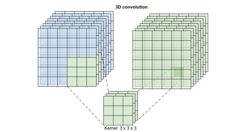
此運算會採用 時間 * 高度 * 寬度 * 通道 輸入，並產生 通道 輸出 (假設輸入和輸出通道的數量相同)。因此，核心大小為 (3 x 3 x 3) 的 3D 卷積層會需要一個權重矩陣，其中包含 27 * 通道 ** 2 個項目。參考論文發現，更有效率且有效的方法是分解卷積。他們提出了一種「(2+1)D」卷積，用於分別處理空間和時間維度，而不是使用單一 3D 卷積來處理時間和空間維度。下圖顯示了 (2 + 1)D 卷積的分解空間和時間卷積。

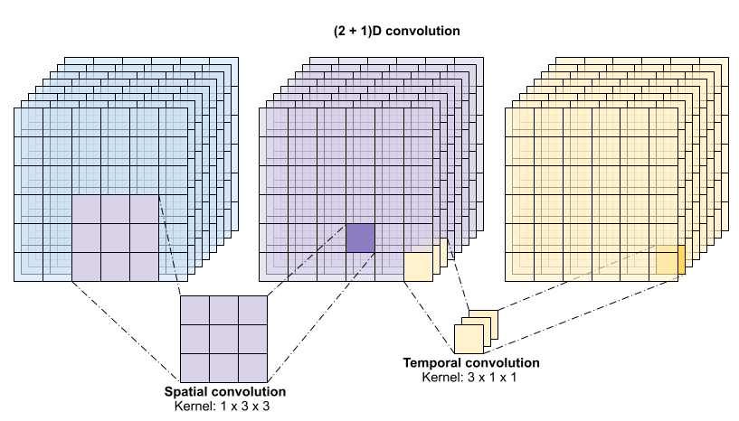
此方法的主要優點是減少參數數量。(2 + 1)D 卷積中的空間卷積會接收形狀為 (1、寬度、高度) 的資料，而時間卷積會接收形狀為 (時間、1、1) 的資料。例如，核心大小為 (3 x 3 x 3) 的 (2 + 1)D 卷積會需要大小為 (9 * 通道**2) + (3 * 通道**2) 的權重矩陣，不到完整 3D 卷積的一半。(2 + 1)D ResNet18 是本教學課程的實作方式，其中 resnet 中的每個卷積都替換為 (2+1)D 卷積。

# Define the dimensions of one frame in the set of frames created
HEIGHT = 224
WIDTH = 224

class Conv2Plus1D(keras.layers.Layer):
  def __init__(self, filters, kernel_size, padding):
    """
      A sequence of convolutional layers that first apply the convolution operation over the
      spatial dimensions, and then the temporal dimension. 
    """
    super().__init__()
    self.seq = keras.Sequential([  
        # Spatial decomposition
        layers.Conv3D(filters=filters,
                      kernel_size=(1, kernel_size[1], kernel_size[2]),
                      padding=padding),
        # Temporal decomposition
        layers.Conv3D(filters=filters, 
                      kernel_size=(kernel_size[0], 1, 1),
                      padding=padding)
        ])

  def call(self, x):
    return self.seq(x)

ResNet 模型由一系列殘差區塊組成。殘差區塊有兩個分支。主要分支執行計算，但梯度難以通過。殘差分支繞過主要計算，主要只是將輸入新增至主要分支的輸出。梯度很容易通過此分支。因此，從損失函數到任何殘差區塊的主要分支都會存在一條簡單的路徑。這避免了梯度消失問題。

使用以下類別建立殘差區塊的主要分支。與標準 ResNet 結構相比，此結構使用自訂 Conv2Plus1D 層，而不是 layers.Conv2D。

class ResidualMain(keras.layers.Layer):
  """
    Residual block of the model with convolution, layer normalization, and the
    activation function, ReLU.
  """
  def __init__(self, filters, kernel_size):
    super().__init__()
    self.seq = keras.Sequential([
        Conv2Plus1D(filters=filters,
                    kernel_size=kernel_size,
                    padding='same'),
        layers.LayerNormalization(),
        layers.ReLU(),
        Conv2Plus1D(filters=filters, 
                    kernel_size=kernel_size,
                    padding='same'),
        layers.LayerNormalization()
    ])

  def call(self, x):
    return self.seq(x)

若要將殘差分支新增至主要分支，則需要具有相同的大小。以下 Project 層處理分支上通道數量變更的情況。特別是，新增了密集連線層序列，後接正規化。

class Project(keras.layers.Layer):
  """
    Project certain dimensions of the tensor as the data is passed through different 
    sized filters and downsampled. 
  """
  def __init__(self, units):
    super().__init__()
    self.seq = keras.Sequential([
        layers.Dense(units),
        layers.LayerNormalization()
    ])

  def call(self, x):
    return self.seq(x)

使用 add_residual_block 在模型的各層之間引入跳躍連線。

def add_residual_block(input, filters, kernel_size):
  """
    Add residual blocks to the model. If the last dimensions of the input data
    and filter size does not match, project it such that last dimension matches.
  """
  out = ResidualMain(filters, 
                     kernel_size)(input)

  res = input
  # Using the Keras functional APIs, project the last dimension of the tensor to
  # match the new filter size
  if out.shape[-1] != input.shape[-1]:
    res = Project(out.shape[-1])(res)

  return layers.add([res, out])

調整影片大小對於執行資料的降取樣是必要的。特別是，對影片影格進行降取樣可讓模型檢查影格的特定部分，以偵測可能特定於特定動作的模式。透過降取樣，可以捨棄非必要的資訊。此外，調整影片大小可減少維度，因此可加快模型的處理速度。

class ResizeVideo(keras.layers.Layer):
  def __init__(self, height, width):
    super().__init__()
    self.height = height
    self.width = width
    self.resizing_layer = layers.Resizing(self.height, self.width)

  def call(self, video):
    """
      Use the einops library to resize the tensor.  

      Args:
        video: Tensor representation of the video, in the form of a set of frames.

      Return:
        A downsampled size of the video according to the new height and width it should be resized to.
    """
    # b stands for batch size, t stands for time, h stands for height, 
    # w stands for width, and c stands for the number of channels.
    old_shape = einops.parse_shape(video, 'b t h w c')
    images = einops.rearrange(video, 'b t h w c -> (b t) h w c')
    images = self.resizing_layer(images)
    videos = einops.rearrange(
        images, '(b t) h w c -> b t h w c',
        t = old_shape['t'])
    return videos

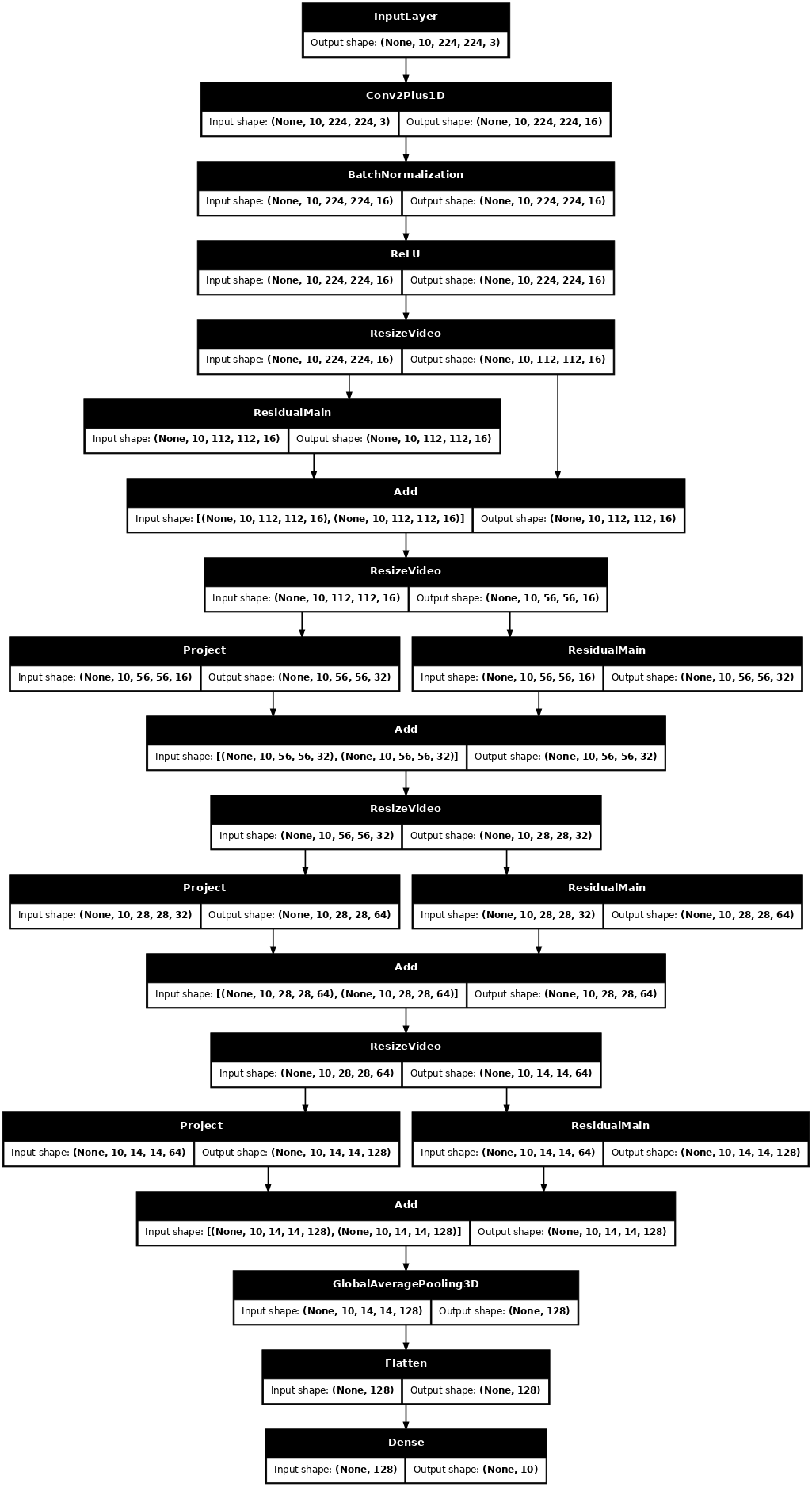
使用 Keras Functional API 建構殘差網路。

input_shape = (None, 10, HEIGHT, WIDTH, 3)
input = layers.Input(shape=(input_shape[1:]))
x = input

x = Conv2Plus1D(filters=16, kernel_size=(3, 7, 7), padding='same')(x)
x = layers.BatchNormalization()(x)
x = layers.ReLU()(x)
x = ResizeVideo(HEIGHT // 2, WIDTH // 2)(x)

# Block 1
x = add_residual_block(x, 16, (3, 3, 3))
x = ResizeVideo(HEIGHT // 4, WIDTH // 4)(x)

# Block 2
x = add_residual_block(x, 32, (3, 3, 3))
x = ResizeVideo(HEIGHT // 8, WIDTH // 8)(x)

# Block 3
x = add_residual_block(x, 64, (3, 3, 3))
x = ResizeVideo(HEIGHT // 16, WIDTH // 16)(x)

# Block 4
x = add_residual_block(x, 128, (3, 3, 3))

x = layers.GlobalAveragePooling3D()(x)
x = layers.Flatten()(x)
x = layers.Dense(10)(x)

model = keras.Model(input, x)

frames, label = next(iter(train_ds))
model.build(frames)

# Visualize the model
keras.utils.plot_model(model, expand_nested=True, dpi=60, show_shapes=True)

訓練模型

在本教學課程中，選擇 tf.keras.optimizers.Adam 最佳化工具和 tf.keras.losses.SparseCategoricalCrossentropy 損失函數。使用 metrics 引數來檢視模型效能在每個步驟的準確度。

model.compile(loss = keras.losses.SparseCategoricalCrossentropy(from_logits=True), 
              optimizer = keras.optimizers.Adam(learning_rate = 0.0001), 
              metrics = ['accuracy'])

使用 Keras Model.fit 方法訓練模型 50 個週期。

history = model.fit(x = train_ds,
                    epochs = 50, 
                    validation_data = val_ds)

Epoch 1/50
WARNING: All log messages before absl::InitializeLog() is called are written to STDERR
I0000 00:00:1720846009.104625  108780 service.cc:146] XLA service 0x7fb998035a60 initialized for platform CUDA (this does not guarantee that XLA will be used). Devices:
I0000 00:00:1720846009.104656  108780 service.cc:154]   StreamExecutor device (0): Tesla T4, Compute Capability 7.5
I0000 00:00:1720846009.104661  108780 service.cc:154]   StreamExecutor device (1): Tesla T4, Compute Capability 7.5
I0000 00:00:1720846009.104665  108780 service.cc:154]   StreamExecutor device (2): Tesla T4, Compute Capability 7.5
I0000 00:00:1720846009.104668  108780 service.cc:154]   StreamExecutor device (3): Tesla T4, Compute Capability 7.5
2024-07-13 04:46:56.420456: E external/local_xla/xla/service/slow_operation_alarm.cc:65] Trying algorithm eng0{} for conv (f32[16,3,1,7,7]{4,3,2,1,0}, u8[0]{0}) custom-call(f32[8,3,10,224,224]{4,3,2,1,0}, f32[8,16,10,224,224]{4,3,2,1,0}), window={size=1x7x7 pad=0_0x3_3x3_3}, dim_labels=bf012_oi012->bf012, custom_call_target="__cudnn$convBackwardFilter", backend_config={"operation_queue_id":"0","wait_on_operation_queues":[],"cudnn_conv_backend_config":{"conv_result_scale":1,"activation_mode":"kNone","side_input_scale":0,"leakyrelu_alpha":0},"force_earliest_schedule":false} is taking a while...
2024-07-13 04:46:56.587823: E external/local_xla/xla/service/slow_operation_alarm.cc:133] The operation took 1.167562786s
Trying algorithm eng0{} for conv (f32[16,3,1,7,7]{4,3,2,1,0}, u8[0]{0}) custom-call(f32[8,3,10,224,224]{4,3,2,1,0}, f32[8,16,10,224,224]{4,3,2,1,0}), window={size=1x7x7 pad=0_0x3_3x3_3}, dim_labels=bf012_oi012->bf012, custom_call_target="__cudnn$convBackwardFilter", backend_config={"operation_queue_id":"0","wait_on_operation_queues":[],"cudnn_conv_backend_config":{"conv_result_scale":1,"activation_mode":"kNone","side_input_scale":0,"leakyrelu_alpha":0},"force_earliest_schedule":false} is taking a while...
I0000 00:00:1720846028.403682  108780 device_compiler.h:188] Compiled cluster using XLA!  This line is logged at most once for the lifetime of the process.
38/Unknown 82s 1s/step - accuracy: 0.1332 - loss: 2.6352
/usr/lib/python3.9/contextlib.py:137: UserWarning: Your input ran out of data; interrupting training. Make sure that your dataset or generator can generate at least `steps_per_epoch * epochs` batches. You may need to use the `.repeat()` function when building your dataset.
  self.gen.throw(typ, value, traceback)
38/38 ━━━━━━━━━━━━━━━━━━━━ 97s 2s/step - accuracy: 0.1328 - loss: 2.6308 - val_accuracy: 0.2000 - val_loss: 2.3839
Epoch 2/50
38/38 ━━━━━━━━━━━━━━━━━━━━ 48s 1s/step - accuracy: 0.1803 - loss: 2.2322 - val_accuracy: 0.1200 - val_loss: 2.3050
Epoch 3/50
38/38 ━━━━━━━━━━━━━━━━━━━━ 48s 1s/step - accuracy: 0.3031 - loss: 2.0525 - val_accuracy: 0.1600 - val_loss: 2.1330
Epoch 4/50
38/38 ━━━━━━━━━━━━━━━━━━━━ 49s 1s/step - accuracy: 0.3243 - loss: 2.0293 - val_accuracy: 0.0900 - val_loss: 2.4266
Epoch 5/50
38/38 ━━━━━━━━━━━━━━━━━━━━ 49s 1s/step - accuracy: 0.2847 - loss: 2.0217 - val_accuracy: 0.3000 - val_loss: 2.0872
Epoch 6/50
38/38 ━━━━━━━━━━━━━━━━━━━━ 49s 1s/step - accuracy: 0.3383 - loss: 1.8919 - val_accuracy: 0.2100 - val_loss: 2.0846
Epoch 7/50
38/38 ━━━━━━━━━━━━━━━━━━━━ 49s 1s/step - accuracy: 0.3150 - loss: 1.7813 - val_accuracy: 0.2400 - val_loss: 2.1339
Epoch 8/50
38/38 ━━━━━━━━━━━━━━━━━━━━ 49s 1s/step - accuracy: 0.3919 - loss: 1.6938 - val_accuracy: 0.3300 - val_loss: 1.9234
Epoch 9/50
38/38 ━━━━━━━━━━━━━━━━━━━━ 49s 1s/step - accuracy: 0.4240 - loss: 1.6314 - val_accuracy: 0.4000 - val_loss: 1.8705
Epoch 10/50
38/38 ━━━━━━━━━━━━━━━━━━━━ 49s 1s/step - accuracy: 0.4294 - loss: 1.6563 - val_accuracy: 0.4200 - val_loss: 1.7679
Epoch 11/50
38/38 ━━━━━━━━━━━━━━━━━━━━ 49s 1s/step - accuracy: 0.4686 - loss: 1.4776 - val_accuracy: 0.4500 - val_loss: 1.6136
Epoch 12/50
38/38 ━━━━━━━━━━━━━━━━━━━━ 49s 1s/step - accuracy: 0.5025 - loss: 1.4471 - val_accuracy: 0.4600 - val_loss: 1.6525
Epoch 13/50
38/38 ━━━━━━━━━━━━━━━━━━━━ 49s 1s/step - accuracy: 0.4857 - loss: 1.3609 - val_accuracy: 0.4100 - val_loss: 1.8119
Epoch 14/50
38/38 ━━━━━━━━━━━━━━━━━━━━ 49s 1s/step - accuracy: 0.4720 - loss: 1.4036 - val_accuracy: 0.4800 - val_loss: 1.6955
Epoch 15/50
38/38 ━━━━━━━━━━━━━━━━━━━━ 49s 1s/step - accuracy: 0.6068 - loss: 1.1491 - val_accuracy: 0.4700 - val_loss: 1.6980
Epoch 16/50
38/38 ━━━━━━━━━━━━━━━━━━━━ 49s 1s/step - accuracy: 0.5794 - loss: 1.1960 - val_accuracy: 0.5300 - val_loss: 1.5192
Epoch 17/50
38/38 ━━━━━━━━━━━━━━━━━━━━ 48s 1s/step - accuracy: 0.5967 - loss: 1.1523 - val_accuracy: 0.5900 - val_loss: 1.3474
Epoch 18/50
38/38 ━━━━━━━━━━━━━━━━━━━━ 48s 1s/step - accuracy: 0.6513 - loss: 0.9858 - val_accuracy: 0.4800 - val_loss: 1.6132
Epoch 19/50
38/38 ━━━━━━━━━━━━━━━━━━━━ 48s 1s/step - accuracy: 0.6359 - loss: 1.0695 - val_accuracy: 0.5800 - val_loss: 1.2987
Epoch 20/50
38/38 ━━━━━━━━━━━━━━━━━━━━ 49s 1s/step - accuracy: 0.6223 - loss: 0.9976 - val_accuracy: 0.6300 - val_loss: 1.2035
Epoch 21/50
38/38 ━━━━━━━━━━━━━━━━━━━━ 48s 1s/step - accuracy: 0.6802 - loss: 0.9198 - val_accuracy: 0.6300 - val_loss: 1.2715
Epoch 22/50
38/38 ━━━━━━━━━━━━━━━━━━━━ 49s 1s/step - accuracy: 0.6602 - loss: 1.0153 - val_accuracy: 0.5900 - val_loss: 1.2321
Epoch 23/50
38/38 ━━━━━━━━━━━━━━━━━━━━ 48s 1s/step - accuracy: 0.7773 - loss: 0.8142 - val_accuracy: 0.5500 - val_loss: 1.5163
Epoch 24/50
38/38 ━━━━━━━━━━━━━━━━━━━━ 49s 1s/step - accuracy: 0.6530 - loss: 0.9162 - val_accuracy: 0.5700 - val_loss: 1.2871
Epoch 25/50
38/38 ━━━━━━━━━━━━━━━━━━━━ 48s 1s/step - accuracy: 0.6627 - loss: 0.8742 - val_accuracy: 0.4200 - val_loss: 1.6656
Epoch 26/50
38/38 ━━━━━━━━━━━━━━━━━━━━ 49s 1s/step - accuracy: 0.6631 - loss: 0.8911 - val_accuracy: 0.5900 - val_loss: 1.1907
Epoch 27/50
38/38 ━━━━━━━━━━━━━━━━━━━━ 49s 1s/step - accuracy: 0.7602 - loss: 0.7582 - val_accuracy: 0.6100 - val_loss: 1.2898
Epoch 28/50
38/38 ━━━━━━━━━━━━━━━━━━━━ 48s 1s/step - accuracy: 0.7274 - loss: 0.8415 - val_accuracy: 0.5800 - val_loss: 1.2001
Epoch 29/50
38/38 ━━━━━━━━━━━━━━━━━━━━ 49s 1s/step - accuracy: 0.7253 - loss: 0.7822 - val_accuracy: 0.6000 - val_loss: 1.1509
Epoch 30/50
38/38 ━━━━━━━━━━━━━━━━━━━━ 48s 1s/step - accuracy: 0.7125 - loss: 0.7782 - val_accuracy: 0.6000 - val_loss: 1.0901
Epoch 31/50
38/38 ━━━━━━━━━━━━━━━━━━━━ 49s 1s/step - accuracy: 0.6901 - loss: 0.8069 - val_accuracy: 0.6500 - val_loss: 1.1331
Epoch 32/50
38/38 ━━━━━━━━━━━━━━━━━━━━ 49s 1s/step - accuracy: 0.7523 - loss: 0.7385 - val_accuracy: 0.6600 - val_loss: 1.1494
Epoch 33/50
38/38 ━━━━━━━━━━━━━━━━━━━━ 49s 1s/step - accuracy: 0.7696 - loss: 0.6941 - val_accuracy: 0.6500 - val_loss: 1.1755
Epoch 34/50
38/38 ━━━━━━━━━━━━━━━━━━━━ 49s 1s/step - accuracy: 0.7705 - loss: 0.6984 - val_accuracy: 0.5900 - val_loss: 1.1887
Epoch 35/50
38/38 ━━━━━━━━━━━━━━━━━━━━ 48s 1s/step - accuracy: 0.7599 - loss: 0.6262 - val_accuracy: 0.5600 - val_loss: 1.1636
Epoch 36/50
38/38 ━━━━━━━━━━━━━━━━━━━━ 49s 1s/step - accuracy: 0.7671 - loss: 0.7025 - val_accuracy: 0.6400 - val_loss: 1.0452
Epoch 37/50
38/38 ━━━━━━━━━━━━━━━━━━━━ 48s 1s/step - accuracy: 0.7253 - loss: 0.7062 - val_accuracy: 0.5900 - val_loss: 1.3652
Epoch 38/50
38/38 ━━━━━━━━━━━━━━━━━━━━ 48s 1s/step - accuracy: 0.7406 - loss: 0.7318 - val_accuracy: 0.6100 - val_loss: 1.1119
Epoch 39/50
38/38 ━━━━━━━━━━━━━━━━━━━━ 49s 1s/step - accuracy: 0.8319 - loss: 0.5269 - val_accuracy: 0.6700 - val_loss: 1.1210
Epoch 40/50
38/38 ━━━━━━━━━━━━━━━━━━━━ 49s 1s/step - accuracy: 0.8297 - loss: 0.5084 - val_accuracy: 0.6300 - val_loss: 1.1432
Epoch 41/50
38/38 ━━━━━━━━━━━━━━━━━━━━ 48s 1s/step - accuracy: 0.7810 - loss: 0.6155 - val_accuracy: 0.4400 - val_loss: 2.0229
Epoch 42/50
38/38 ━━━━━━━━━━━━━━━━━━━━ 48s 1s/step - accuracy: 0.7794 - loss: 0.7254 - val_accuracy: 0.5500 - val_loss: 1.3363
Epoch 43/50
38/38 ━━━━━━━━━━━━━━━━━━━━ 49s 1s/step - accuracy: 0.7729 - loss: 0.6237 - val_accuracy: 0.5100 - val_loss: 1.4360
Epoch 44/50
38/38 ━━━━━━━━━━━━━━━━━━━━ 49s 1s/step - accuracy: 0.8165 - loss: 0.5819 - val_accuracy: 0.6000 - val_loss: 1.1835
Epoch 45/50
38/38 ━━━━━━━━━━━━━━━━━━━━ 49s 1s/step - accuracy: 0.8340 - loss: 0.5026 - val_accuracy: 0.6400 - val_loss: 1.1179
Epoch 46/50
38/38 ━━━━━━━━━━━━━━━━━━━━ 48s 1s/step - accuracy: 0.8695 - loss: 0.4977 - val_accuracy: 0.6100 - val_loss: 1.0725
Epoch 47/50
38/38 ━━━━━━━━━━━━━━━━━━━━ 48s 1s/step - accuracy: 0.8564 - loss: 0.4611 - val_accuracy: 0.6600 - val_loss: 1.1611
Epoch 48/50
38/38 ━━━━━━━━━━━━━━━━━━━━ 49s 1s/step - accuracy: 0.8388 - loss: 0.5222 - val_accuracy: 0.5900 - val_loss: 1.2520
Epoch 49/50
38/38 ━━━━━━━━━━━━━━━━━━━━ 48s 1s/step - accuracy: 0.8233 - loss: 0.5380 - val_accuracy: 0.6400 - val_loss: 1.0974
Epoch 50/50
38/38 ━━━━━━━━━━━━━━━━━━━━ 48s 1s/step - accuracy: 0.8523 - loss: 0.4805 - val_accuracy: 0.6300 - val_loss: 1.1175

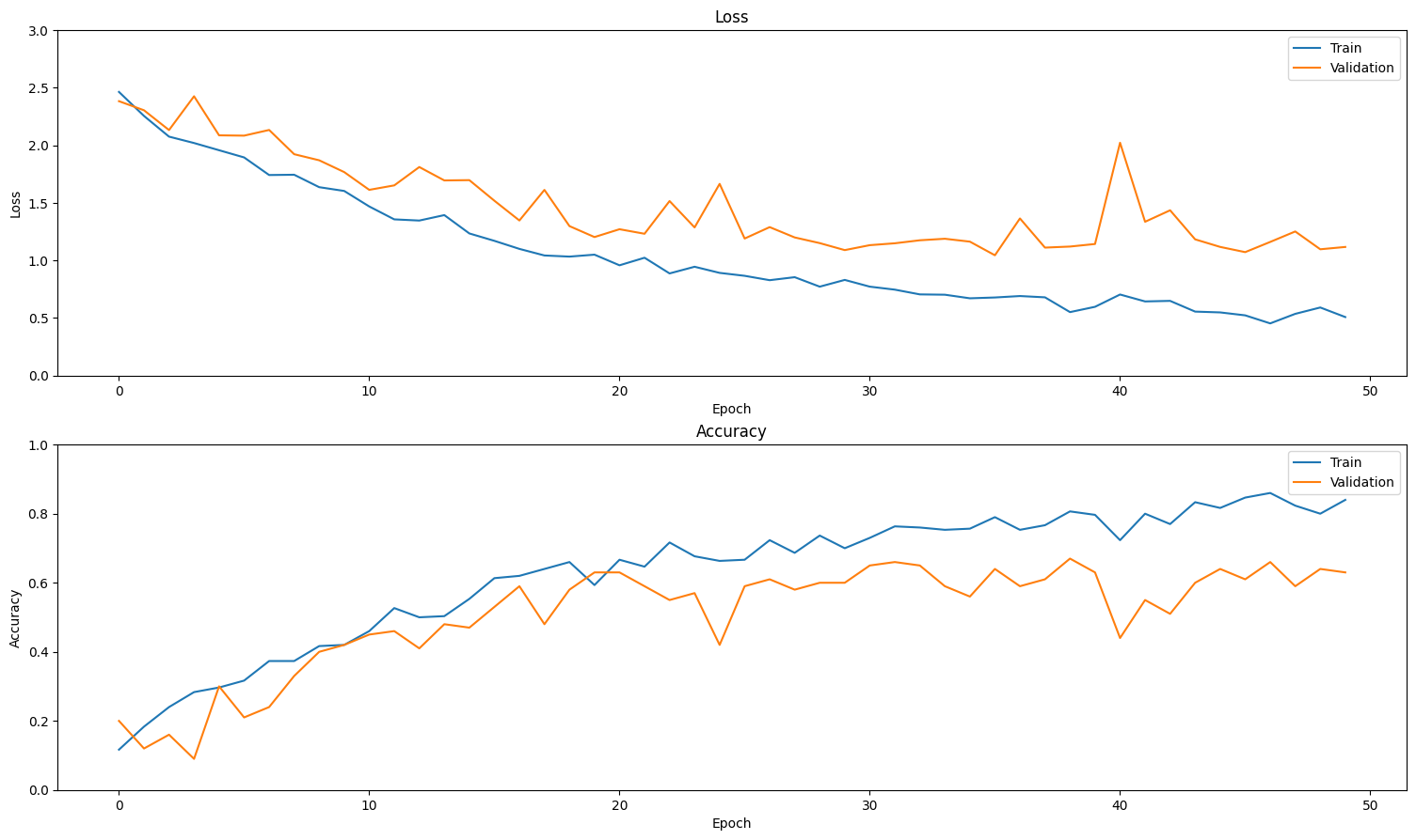
視覺化結果

建立訓練集和驗證集的損失和準確度圖表

def plot_history(history):
  """
    Plotting training and validation learning curves.

    Args:
      history: model history with all the metric measures
  """
  fig, (ax1, ax2) = plt.subplots(2)

  fig.set_size_inches(18.5, 10.5)

  # Plot loss
  ax1.set_title('Loss')
  ax1.plot(history.history['loss'], label = 'train')
  ax1.plot(history.history['val_loss'], label = 'test')
  ax1.set_ylabel('Loss')

  # Determine upper bound of y-axis
  max_loss = max(history.history['loss'] + history.history['val_loss'])

  ax1.set_ylim([0, np.ceil(max_loss)])
  ax1.set_xlabel('Epoch')
  ax1.legend(['Train', 'Validation']) 

  # Plot accuracy
  ax2.set_title('Accuracy')
  ax2.plot(history.history['accuracy'],  label = 'train')
  ax2.plot(history.history['val_accuracy'], label = 'test')
  ax2.set_ylabel('Accuracy')
  ax2.set_ylim([0, 1])
  ax2.set_xlabel('Epoch')
  ax2.legend(['Train', 'Validation'])

  plt.show()

plot_history(history)

評估模型

使用 Keras Model.evaluate 取得測試資料集的損失和準確度。

model.evaluate(test_ds, return_dict=True)

13/13 ━━━━━━━━━━━━━━━━━━━━ 11s 844ms/step - accuracy: 0.4477 - loss: 1.2893
{'accuracy': 0.5099999904632568, 'loss': 1.2706645727157593}

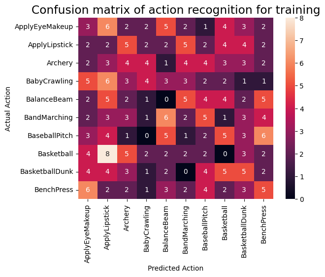
若要進一步視覺化模型效能，請使用混淆矩陣。混淆矩陣可讓您評估分類模型的效能，而不僅僅是準確度。為了針對此多類別分類問題建構混淆矩陣，請取得測試集中的實際值和預測值。

def get_actual_predicted_labels(dataset): 
  """
    Create a list of actual ground truth values and the predictions from the model.

    Args:
      dataset: An iterable data structure, such as a TensorFlow Dataset, with features and labels.

    Return:
      Ground truth and predicted values for a particular dataset.
  """
  actual = [labels for _, labels in dataset.unbatch()]
  predicted = model.predict(dataset)

  actual = tf.stack(actual, axis=0)
  predicted = tf.concat(predicted, axis=0)
  predicted = tf.argmax(predicted, axis=1)

  return actual, predicted

def plot_confusion_matrix(actual, predicted, labels, ds_type):
  cm = tf.math.confusion_matrix(actual, predicted)
  ax = sns.heatmap(cm, annot=True, fmt='g')
  sns.set(rc={'figure.figsize':(12, 12)})
  sns.set(font_scale=1.4)
  ax.set_title('Confusion matrix of action recognition for ' + ds_type)
  ax.set_xlabel('Predicted Action')
  ax.set_ylabel('Actual Action')
  plt.xticks(rotation=90)
  plt.yticks(rotation=0)
  ax.xaxis.set_ticklabels(labels)
  ax.yaxis.set_ticklabels(labels)

fg = FrameGenerator(subset_paths['train'], n_frames, training=True)
labels = list(fg.class_ids_for_name.keys())

actual, predicted = get_actual_predicted_labels(train_ds)
plot_confusion_matrix(actual, predicted, labels, 'training')

38/38 ━━━━━━━━━━━━━━━━━━━━ 35s 877ms/step

actual, predicted = get_actual_predicted_labels(test_ds)
plot_confusion_matrix(actual, predicted, labels, 'test')

13/13 ━━━━━━━━━━━━━━━━━━━━ 11s 831ms/step
/usr/lib/python3.9/contextlib.py:137: UserWarning: Your input ran out of data; interrupting training. Make sure that your dataset or generator can generate at least `steps_per_epoch * epochs` batches. You may need to use the `.repeat()` function when building your dataset.
  self.gen.throw(typ, value, traceback)

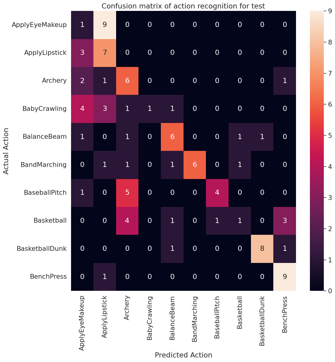
每個類別的精確度和召回率值也可以使用混淆矩陣計算。

def calculate_classification_metrics(y_actual, y_pred, labels):
  """
    Calculate the precision and recall of a classification model using the ground truth and
    predicted values. 

    Args:
      y_actual: Ground truth labels.
      y_pred: Predicted labels.
      labels: List of classification labels.

    Return:
      Precision and recall measures.
  """
  cm = tf.math.confusion_matrix(y_actual, y_pred)
  tp = np.diag(cm) # Diagonal represents true positives
  precision = dict()
  recall = dict()
  for i in range(len(labels)):
    col = cm[:, i]
    fp = np.sum(col) - tp[i] # Sum of column minus true positive is false negative

    row = cm[i, :]
    fn = np.sum(row) - tp[i] # Sum of row minus true positive, is false negative

    precision[labels[i]] = tp[i] / (tp[i] + fp) # Precision 

    recall[labels[i]] = tp[i] / (tp[i] + fn) # Recall

  return precision, recall

precision, recall = calculate_classification_metrics(actual, predicted, labels) # Test dataset

precision

{'ApplyEyeMakeup': 0.08333333333333333,
 'ApplyLipstick': 0.3181818181818182,
 'Archery': 0.3333333333333333,
 'BabyCrawling': 1.0,
 'BalanceBeam': 0.6,
 'BandMarching': 1.0,
 'BaseballPitch': 0.8,
 'Basketball': 0.3333333333333333,
 'BasketballDunk': 0.8888888888888888,
 'BenchPress': 0.6428571428571429}

recall

{'ApplyEyeMakeup': 0.1,
 'ApplyLipstick': 0.7,
 'Archery': 0.6,
 'BabyCrawling': 0.1,
 'BalanceBeam': 0.6,
 'BandMarching': 0.6,
 'BaseballPitch': 0.4,
 'Basketball': 0.1,
 'BasketballDunk': 0.8,
 'BenchPress': 0.9}

後續步驟

若要進一步瞭解如何在 TensorFlow 中使用影片資料，請查看以下教學課程：

• 載入影片資料
• 用於串流動作辨識的 MoViNet
• 使用 MoViNet 進行影片分類遷移學習