
|
|
|
 在 GitHub 上檢視原始碼 在 GitHub 上檢視原始碼
|
|
本教學課程簡介如何使用 TensorFlow 進行時間序列預測。它會建構幾種不同的模型樣式,包括卷積神經網路和循環神經網路 (CNN 和 RNN)。
本教學課程涵蓋兩個主要部分,以及子章節
- 單一步驟的時間序列預測
- 單一特徵。
- 所有特徵。
- 多步驟的時間序列預測
- 單次完成:一次完成所有預測。
- 自動迴歸:一次預測一個值,並將輸出結果饋送回模型。
設定
import os
import datetime

import IPython
import IPython.display
import matplotlib as mpl
import matplotlib.pyplot as plt
import numpy as np
import pandas as pd
import seaborn as sns
import tensorflow as tf

mpl.rcParams['figure.figsize'] = (8, 6)
mpl.rcParams['axes.grid'] = False
2024-06-30 02:52:03.533068: E external/local_xla/xla/stream_executor/cuda/cuda_fft.cc:479] Unable to register cuFFT factory: Attempting to register factory for plugin cuFFT when one has already been registered
2024-06-30 02:52:03.558530: E external/local_xla/xla/stream_executor/cuda/cuda_dnn.cc:10575] Unable to register cuDNN factory: Attempting to register factory for plugin cuDNN when one has already been registered
2024-06-30 02:52:03.558567: E external/local_xla/xla/stream_executor/cuda/cuda_blas.cc:1442] Unable to register cuBLAS factory: Attempting to register factory for plugin cuBLAS when one has already been registered
氣象資料集
本教學課程使用 氣象時間序列資料集,由 Max Planck Institute for Biogeochemistry 錄製。
這個資料集包含 14 種不同的特徵,例如氣溫、大氣壓力和濕度。這些資料從 2003 年開始每 10 分鐘收集一次。為了提高效率,您將只使用 2009 年到 2016 年之間收集的資料。 François Chollet 為其著作 Deep Learning with Python 準備了這個資料集區段。
zip_path = tf.keras.utils.get_file(
    origin='https://storage.googleapis.com/tensorflow/tf-keras-datasets/jena_climate_2009_2016.csv.zip',
    fname='jena_climate_2009_2016.csv.zip',
    extract=True)
csv_path, _ = os.path.splitext(zip_path)
Downloading data from https://storage.googleapis.com/tensorflow/tf-keras-datasets/jena_climate_2009_2016.csv.zip
13568290/13568290 ━━━━━━━━━━━━━━━━━━━━ 0s 0us/step
本教學課程只會處理每小時預測,因此首先將資料從 10 分鐘間隔子取樣為一小時間隔
df = pd.read_csv(csv_path)
# Slice [start:stop:step], starting from index 5 take every 6th record.
df = df[5::6]

date_time = pd.to_datetime(df.pop('Date Time'), format='%d.%m.%Y %H:%M:%S')
讓我們快速瀏覽一下資料。以下是前幾列
df.head()
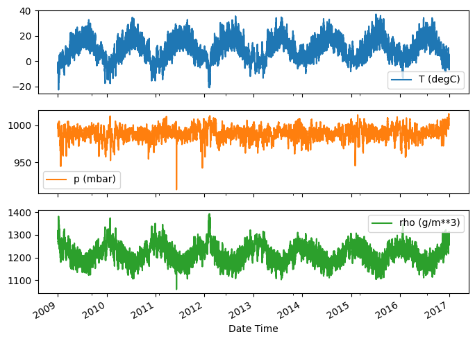
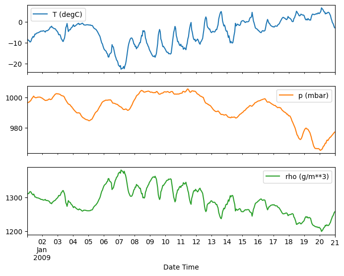
以下是一些特徵隨時間演進的狀況
plot_cols = ['T (degC)', 'p (mbar)', 'rho (g/m**3)']
plot_features = df[plot_cols]
plot_features.index = date_time
_ = plot_features.plot(subplots=True)

plot_features = df[plot_cols][:480]
plot_features.index = date_time[:480]
_ = plot_features.plot(subplots=True)
檢查與清理
接下來,查看資料集的統計資料
df.describe().transpose()
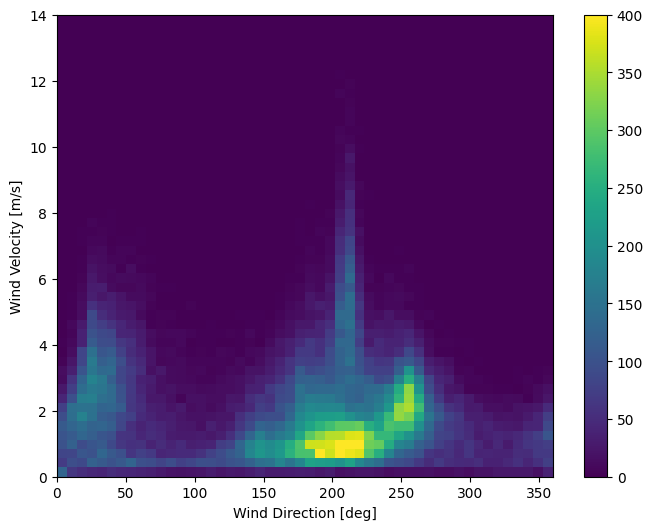
風速
其中一件應該注意到的事情是風速 (wv (m/s)) 和最大風速 (max. wv (m/s)) 欄的 min 值。這個 -9999 很可能是錯誤的。
有一個獨立的風向欄,因此風速應大於零 (>=0)。將其取代為零
wv = df['wv (m/s)']
bad_wv = wv == -9999.0
wv[bad_wv] = 0.0

max_wv = df['max. wv (m/s)']
bad_max_wv = max_wv == -9999.0
max_wv[bad_max_wv] = 0.0

# The above inplace edits are reflected in the DataFrame.
df['wv (m/s)'].min()
0.0
特徵工程
在深入建構模型之前,務必先瞭解您的資料,並確保您將格式正確的資料傳遞給模型。
風
資料的最後一欄 wd (deg)—以度為單位表示風向。角度不是好的模型輸入:360° 和 0° 應該彼此接近,並且平滑地環繞。如果沒有風,則方向應該無關緊要。
目前,風資料的分佈看起來像這樣
plt.hist2d(df['wd (deg)'], df['wv (m/s)'], bins=(50, 50), vmax=400)
plt.colorbar()
plt.xlabel('Wind Direction [deg]')
plt.ylabel('Wind Velocity [m/s]')
Text(0, 0.5, 'Wind Velocity [m/s]')
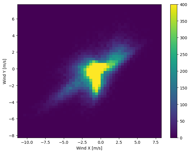
但是,如果您將風向和風速欄轉換為風向量,模型會更容易解讀
wv = df.pop('wv (m/s)')
max_wv = df.pop('max. wv (m/s)')

# Convert to radians.
wd_rad = df.pop('wd (deg)')*np.pi / 180

# Calculate the wind x and y components.
df['Wx'] = wv*np.cos(wd_rad)
df['Wy'] = wv*np.sin(wd_rad)

# Calculate the max wind x and y components.
df['max Wx'] = max_wv*np.cos(wd_rad)
df['max Wy'] = max_wv*np.sin(wd_rad)
風向量的分佈對模型來說更容易正確解讀
plt.hist2d(df['Wx'], df['Wy'], bins=(50, 50), vmax=400)
plt.colorbar()
plt.xlabel('Wind X [m/s]')
plt.ylabel('Wind Y [m/s]')
ax = plt.gca()
ax.axis('tight')
(-11.305513973134667, 8.24469928549079, -8.27438540335515, 7.7338312955467785)
時間
同樣地,Date Time 欄非常有用,但不適用於這種字串形式。首先將其轉換為秒
timestamp_s = date_time.map(pd.Timestamp.timestamp)
與風向類似,以秒為單位表示的時間不是有用的模型輸入。由於是氣象資料,因此具有明顯的每日和每年週期性。有很多方法可以處理週期性。
您可以使用正弦和餘弦轉換來清除「一天中的時間」和「一年中的時間」訊號,以取得可用的訊號
day = 24*60*60
year = (365.2425)*day

df['Day sin'] = np.sin(timestamp_s * (2 * np.pi / day))
df['Day cos'] = np.cos(timestamp_s * (2 * np.pi / day))
df['Year sin'] = np.sin(timestamp_s * (2 * np.pi / year))
df['Year cos'] = np.cos(timestamp_s * (2 * np.pi / year))
plt.plot(np.array(df['Day sin'])[:25])
plt.plot(np.array(df['Day cos'])[:25])
plt.xlabel('Time [h]')
plt.title('Time of day signal')
Text(0.5, 1.0, 'Time of day signal')
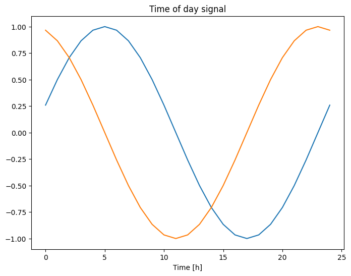
這讓模型能夠存取最重要的頻率特徵。在本例中,您事先知道哪些頻率很重要。
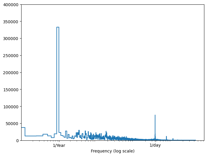
如果您沒有該資訊,您可以透過使用 快速傅立葉轉換 擷取特徵來判斷哪些頻率很重要。為了檢查假設,以下是溫度隨時間變化的 tf.signal.rfft。請注意,在接近 1/year 和 1/day 的頻率處有明顯的峰值
fft = tf.signal.rfft(df['T (degC)'])
f_per_dataset = np.arange(0, len(fft))

n_samples_h = len(df['T (degC)'])
hours_per_year = 24*365.2524
years_per_dataset = n_samples_h/(hours_per_year)

f_per_year = f_per_dataset/years_per_dataset
plt.step(f_per_year, np.abs(fft))
plt.xscale('log')
plt.ylim(0, 400000)
plt.xlim([0.1, max(plt.xlim())])
plt.xticks([1, 365.2524], labels=['1/Year', '1/day'])
_ = plt.xlabel('Frequency (log scale)')
分割資料
您將使用 (70%, 20%, 10%) 分割來分割訓練、驗證和測試集。請注意,資料在分割前不會隨機洗牌。這有兩個原因
- 它確保將資料切割成連續樣本的視窗仍然可行。
- 它確保驗證/測試結果更真實,因為是在模型訓練後收集的資料上進行評估。
column_indices = {name: i for i, name in enumerate(df.columns)}

n = len(df)
train_df = df[0:int(n*0.7)]
val_df = df[int(n*0.7):int(n*0.9)]
test_df = df[int(n*0.9):]

num_features = df.shape[1]
正規化資料
在訓練神經網路之前,縮放特徵非常重要。正規化是執行此縮放的常用方法:減去每個特徵的平均值,然後除以標準差。
平均值和標準差應僅使用訓練資料計算,以便模型無法存取驗證集和測試集中的值。
此外,模型在訓練時不應存取訓練集中的未來值,並且此正規化應使用移動平均值完成,這也是值得爭論的。這不是本教學課程的重點,而驗證集和測試集可確保您獲得 (在某種程度上) 誠實的指標。因此,為了簡化起見,本教學課程使用簡單的平均值。
train_mean = train_df.mean()
train_std = train_df.std()

train_df = (train_df - train_mean) / train_std
val_df = (val_df - train_mean) / train_std
test_df = (test_df - train_mean) / train_std
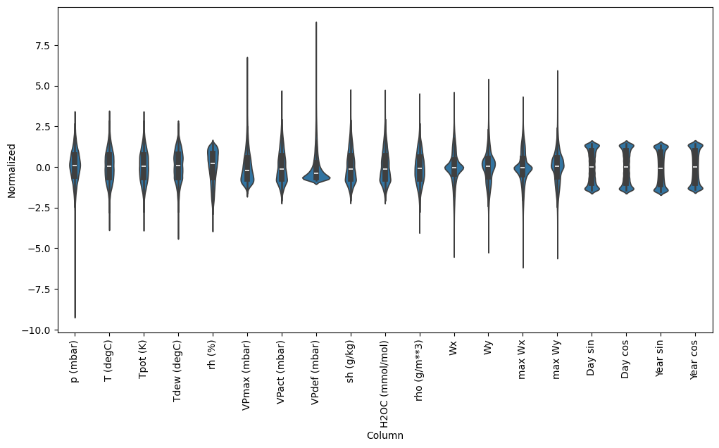
現在,快速查看特徵的分佈。有些特徵確實具有長尾,但沒有像 -9999 風速值那樣的明顯錯誤。
df_std = (df - train_mean) / train_std
df_std = df_std.melt(var_name='Column', value_name='Normalized')
plt.figure(figsize=(12, 6))
ax = sns.violinplot(x='Column', y='Normalized', data=df_std)
_ = ax.set_xticklabels(df.keys(), rotation=90)
/tmpfs/tmp/ipykernel_117798/3214313372.py:5: UserWarning: set_ticklabels() should only be used with a fixed number of ticks, i.e. after set_ticks() or using a FixedLocator.
  _ = ax.set_xticklabels(df.keys(), rotation=90)
資料視窗化
本教學課程中的模型將根據資料中連續樣本的視窗進行一組預測。
輸入視窗的主要特徵如下
- 輸入和標籤視窗的寬度 (時間步數)。
- 它們之間的時間偏移。
- 哪些特徵用作輸入、標籤或兩者。
本教學課程建構各種模型 (包括線性、DNN、CNN 和 RNN 模型),並將其用於
- 單一輸出和多輸出預測。
- 單一時間步和多時間步預測。
本節重點說明資料視窗化的實作方式,以便它可以重複用於所有這些模型。
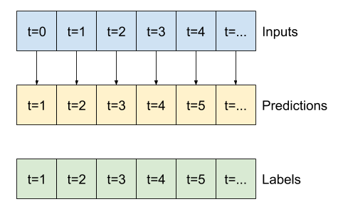
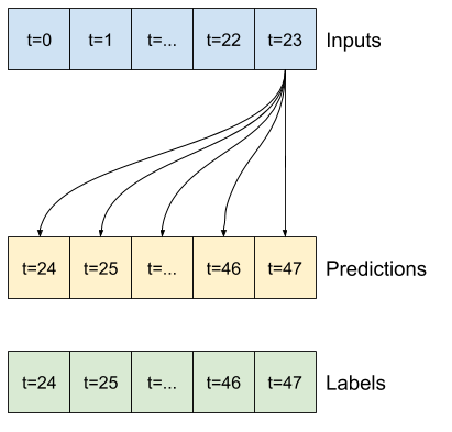
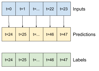
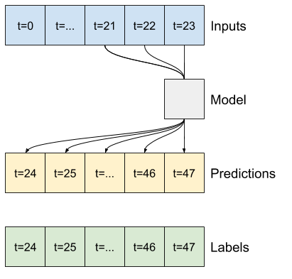
根據任務和模型類型,您可能想要產生各種資料視窗。以下是一些範例
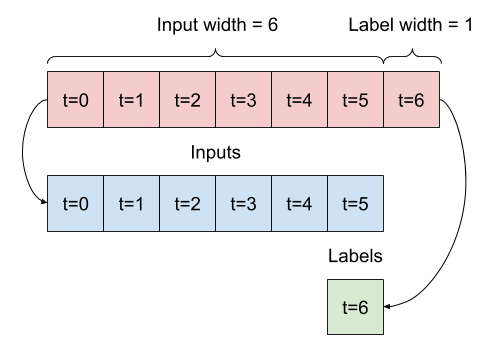
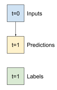
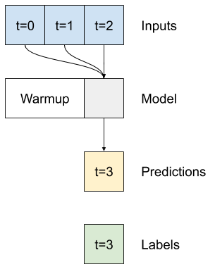
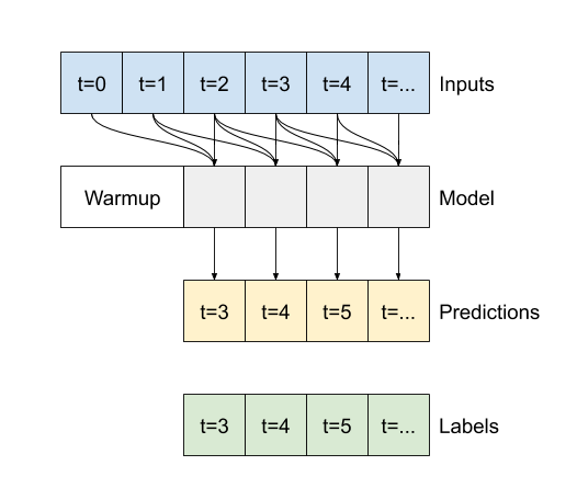
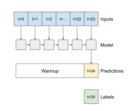
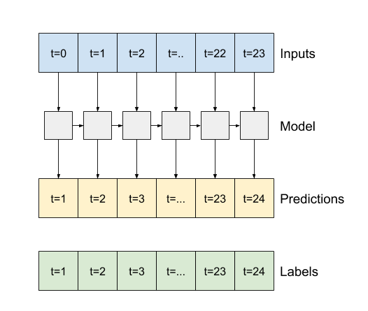
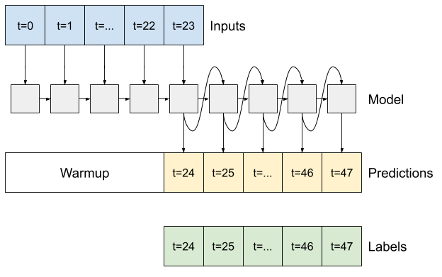
例如,若要根據 24 小時的歷史記錄,預測未來 24 小時的單一預測,您可以定義如下的視窗

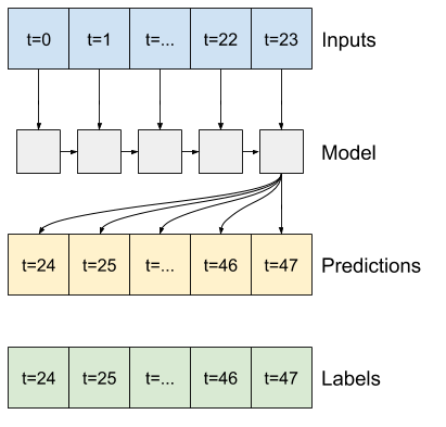
一個模型根據六小時的歷史記錄,預測未來一小時的預測,則需要如下的視窗
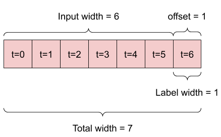
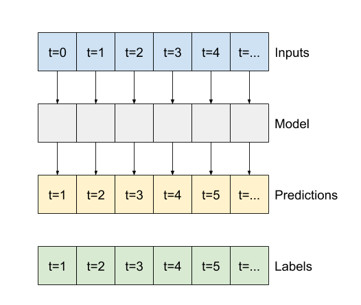
本節的其餘部分定義了 WindowGenerator 類別。此類別可以
- 處理索引和偏移,如上圖所示。
- 將特徵視窗分割為
(features, labels)配對。 - 繪製結果視窗的內容。
- 使用
tf.data.Dataset,從訓練、評估和測試資料有效率地產生這些視窗的批次。
1. 索引和偏移
首先建立 WindowGenerator 類別。__init__ 方法包含輸入和標籤索引的所有必要邏輯。
它也會將訓練、評估和測試 DataFrame 作為輸入。這些稍後將轉換為視窗的 tf.data.Dataset。
class WindowGenerator():
  def __init__(self, input_width, label_width, shift,
               train_df=train_df, val_df=val_df, test_df=test_df,
               label_columns=None):
    # Store the raw data.
    self.train_df = train_df
    self.val_df = val_df
    self.test_df = test_df

    # Work out the label column indices.
    self.label_columns = label_columns
    if label_columns is not None:
      self.label_columns_indices = {name: i for i, name in
                                    enumerate(label_columns)}
    self.column_indices = {name: i for i, name in
                           enumerate(train_df.columns)}

    # Work out the window parameters.
    self.input_width = input_width
    self.label_width = label_width
    self.shift = shift

    self.total_window_size = input_width + shift

    self.input_slice = slice(0, input_width)
    self.input_indices = np.arange(self.total_window_size)[self.input_slice]

    self.label_start = self.total_window_size - self.label_width
    self.labels_slice = slice(self.label_start, None)
    self.label_indices = np.arange(self.total_window_size)[self.labels_slice]

  def __repr__(self):
    return '\n'.join([
        f'Total window size: {self.total_window_size}',
        f'Input indices: {self.input_indices}',
        f'Label indices: {self.label_indices}',
        f'Label column name(s): {self.label_columns}'])
以下是在本節開頭圖表中顯示的 2 個視窗的建立程式碼
w1 = WindowGenerator(input_width=24, label_width=1, shift=24,
                     label_columns=['T (degC)'])
w1
Total window size: 48
Input indices: [ 0  1  2  3  4  5  6  7  8  9 10 11 12 13 14 15 16 17 18 19 20 21 22 23]
Label indices: [47]
Label column name(s): ['T (degC)']
w2 = WindowGenerator(input_width=6, label_width=1, shift=1,
                     label_columns=['T (degC)'])
w2
Total window size: 7
Input indices: [0 1 2 3 4 5]
Label indices: [6]
Label column name(s): ['T (degC)']
2. 分割
給定連續輸入的清單,split_window 方法會將它們轉換為輸入視窗和標籤視窗。
您稍早定義的範例 w2 將會像這樣分割
此圖表未顯示資料的 features 軸,但此 split_window 函式也會處理 label_columns,因此它可以同時用於單一輸出和多輸出範例。
def split_window(self, features):
  inputs = features[:, self.input_slice, :]
  labels = features[:, self.labels_slice, :]
  if self.label_columns is not None:
    labels = tf.stack(
        [labels[:, :, self.column_indices[name]] for name in self.label_columns],
        axis=-1)

  # Slicing doesn't preserve static shape information, so set the shapes
  # manually. This way the `tf.data.Datasets` are easier to inspect.
  inputs.set_shape([None, self.input_width, None])
  labels.set_shape([None, self.label_width, None])

  return inputs, labels

WindowGenerator.split_window = split_window
試用看看
# Stack three slices, the length of the total window.
example_window = tf.stack([np.array(train_df[:w2.total_window_size]),
                           np.array(train_df[100:100+w2.total_window_size]),
                           np.array(train_df[200:200+w2.total_window_size])])

example_inputs, example_labels = w2.split_window(example_window)

print('All shapes are: (batch, time, features)')
print(f'Window shape: {example_window.shape}')
print(f'Inputs shape: {example_inputs.shape}')
print(f'Labels shape: {example_labels.shape}')
All shapes are: (batch, time, features)
Window shape: (3, 7, 19)
Inputs shape: (3, 6, 19)
Labels shape: (3, 1, 1)
一般來說,TensorFlow 中的資料會封裝成陣列,其中最外層的索引是跨範例 (「批次」維度)。中間的索引是「時間」或「空間」(寬度、高度) 維度。最內層的索引是特徵。
上面的程式碼採用了由三個 7 時間步視窗組成的批次,每個時間步都有 19 個特徵。它將它們分割成一個由 6 時間步 19 特徵輸入組成的批次,以及一個 1 時間步 1 特徵標籤。標籤只有一個特徵,因為 WindowGenerator 是使用 label_columns=['T (degC)'] 初始化的。最初,本教學課程將建構預測單一輸出標籤的模型。
3. 繪圖
以下是一個繪圖方法,可讓您簡單地視覺化分割視窗
w2.example = example_inputs, example_labels
def plot(self, model=None, plot_col='T (degC)', max_subplots=3):
  inputs, labels = self.example
  plt.figure(figsize=(12, 8))
  plot_col_index = self.column_indices[plot_col]
  max_n = min(max_subplots, len(inputs))
  for n in range(max_n):
    plt.subplot(max_n, 1, n+1)
    plt.ylabel(f'{plot_col} [normed]')
    plt.plot(self.input_indices, inputs[n, :, plot_col_index],
             label='Inputs', marker='.', zorder=-10)

    if self.label_columns:
      label_col_index = self.label_columns_indices.get(plot_col, None)
    else:
      label_col_index = plot_col_index

    if label_col_index is None:
      continue

    plt.scatter(self.label_indices, labels[n, :, label_col_index],
                edgecolors='k', label='Labels', c='#2ca02c', s=64)
    if model is not None:
      predictions = model(inputs)
      plt.scatter(self.label_indices, predictions[n, :, label_col_index],
                  marker='X', edgecolors='k', label='Predictions',
                  c='#ff7f0e', s=64)

    if n == 0:
      plt.legend()

  plt.xlabel('Time [h]')

WindowGenerator.plot = plot
此繪圖會根據項目參考的時間對齊輸入、標籤和 (稍後的) 預測
w2.plot()
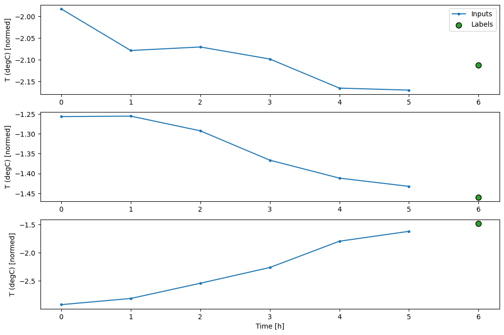
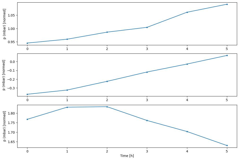
您可以繪製其他欄,但範例視窗 w2 設定僅針對 T (degC) 欄具有標籤。
w2.plot(plot_col='p (mbar)')
4. 建立 tf.data.Dataset
最後,此 make_dataset 方法會採用時間序列 DataFrame,並使用您定義的 tf.keras.utils.timeseries_dataset_from_array 函式,將其轉換為 (input_window, label_window) 配對的 tf.data.Dataset
def make_dataset(self, data):
  data = np.array(data, dtype=np.float32)
  ds = tf.keras.utils.timeseries_dataset_from_array(
      data=data,
      targets=None,
      sequence_length=self.total_window_size,
      sequence_stride=1,
      shuffle=True,
      batch_size=32,)

  ds = ds.map(self.split_window)

  return ds

WindowGenerator.make_dataset = make_dataset
WindowGenerator 物件會保留訓練、驗證和測試資料。
新增屬性,以使用您稍早定義的 make_dataset 方法,將它們作為 tf.data.Dataset 存取。此外,新增標準範例批次以便於存取和繪圖
@property
def train(self):
  return self.make_dataset(self.train_df)

@property
def val(self):
  return self.make_dataset(self.val_df)

@property
def test(self):
  return self.make_dataset(self.test_df)

@property
def example(self):
  """Get and cache an example batch of `inputs, labels` for plotting."""
  result = getattr(self, '_example', None)
  if result is None:
    # No example batch was found, so get one from the `.train` dataset
    result = next(iter(self.train))
    # And cache it for next time
    self._example = result
  return result

WindowGenerator.train = train
WindowGenerator.val = val
WindowGenerator.test = test
WindowGenerator.example = example
現在,WindowGenerator 物件可讓您存取 tf.data.Dataset 物件,因此您可以輕鬆地逐一查看資料。
Dataset.element_spec 屬性會告訴您資料集元素的結構、資料類型和形狀。
# Each element is an (inputs, label) pair.
w2.train.element_spec
(TensorSpec(shape=(None, 6, 19), dtype=tf.float32, name=None),
 TensorSpec(shape=(None, 1, 1), dtype=tf.float32, name=None))
逐一查看 Dataset 會產生具體批次
for example_inputs, example_labels in w2.train.take(1):
  print(f'Inputs shape (batch, time, features): {example_inputs.shape}')
  print(f'Labels shape (batch, time, features): {example_labels.shape}')
Inputs shape (batch, time, features): (32, 6, 19)
Labels shape (batch, time, features): (32, 1, 1)
2024-06-30 02:52:21.131505: W tensorflow/core/framework/local_rendezvous.cc:404] Local rendezvous is aborting with status: OUT_OF_RANGE: End of sequence
單一步驟模型
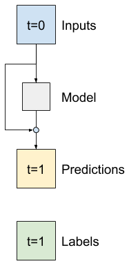
您可以根據這類資料建構的最簡單模型,是根據目前條件預測單一特徵值 (未來 1 個時間步 (一小時)) 的模型。
因此,首先建構模型來預測未來一小時的 T (degC) 值。
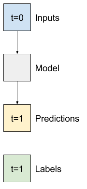
設定 WindowGenerator 物件,以產生這些單一步驟 (input, label) 配對
single_step_window = WindowGenerator(
    input_width=1, label_width=1, shift=1,
    label_columns=['T (degC)'])
single_step_window
Total window size: 2
Input indices: [0]
Label indices: [1]
Label column name(s): ['T (degC)']
window 物件會從訓練、驗證和測試集建立 tf.data.Dataset,讓您可以輕鬆地逐一查看資料批次。
for example_inputs, example_labels in single_step_window.train.take(1):
  print(f'Inputs shape (batch, time, features): {example_inputs.shape}')
  print(f'Labels shape (batch, time, features): {example_labels.shape}')
Inputs shape (batch, time, features): (32, 1, 19)
Labels shape (batch, time, features): (32, 1, 1)
2024-06-30 02:52:21.281467: W tensorflow/core/framework/local_rendezvous.cc:404] Local rendezvous is aborting with status: OUT_OF_RANGE: End of sequence
基準
在建構可訓練模型之前,最好先有一個效能基準,作為與稍後更複雜的模型比較的點。
第一個任務是根據所有特徵的目前值,預測未來一小時的溫度。目前值包括目前的溫度。
因此,從一個只傳回目前溫度作為預測的模型開始,預測「沒有變化」。這是一個合理的基準,因為溫度變化緩慢。當然,如果您預測更遙遠的未來,此基準的效果會比較差。
class Baseline(tf.keras.Model):
  def __init__(self, label_index=None):
    super().__init__()
    self.label_index = label_index

  def call(self, inputs):
    if self.label_index is None:
      return inputs
    result = inputs[:, :, self.label_index]
    return result[:, :, tf.newaxis]
例項化並評估此模型
baseline = Baseline(label_index=column_indices['T (degC)'])

baseline.compile(loss=tf.keras.losses.MeanSquaredError(),
                 metrics=[tf.keras.metrics.MeanAbsoluteError()])

val_performance = {}
performance = {}
val_performance['Baseline'] = baseline.evaluate(single_step_window.val, return_dict=True)
performance['Baseline'] = baseline.evaluate(single_step_window.test, verbose=0, return_dict=True)
1/439 ━━━━━━━━━━━━━━━━━━━━ 2:24 330ms/step - loss: 0.0173 - mean_absolute_error: 0.0970
WARNING: All log messages before absl::InitializeLog() is called are written to STDERR
I0000 00:00:1719715941.527831  117969 service.cc:145] XLA service 0x7f1550004690 initialized for platform CUDA (this does not guarantee that XLA will be used). Devices:
I0000 00:00:1719715941.527904  117969 service.cc:153]   StreamExecutor device (0): Tesla T4, Compute Capability 7.5
I0000 00:00:1719715941.527913  117969 service.cc:153]   StreamExecutor device (1): Tesla T4, Compute Capability 7.5
I0000 00:00:1719715941.527919  117969 service.cc:153]   StreamExecutor device (2): Tesla T4, Compute Capability 7.5
I0000 00:00:1719715941.527925  117969 service.cc:153]   StreamExecutor device (3): Tesla T4, Compute Capability 7.5
I0000 00:00:1719715941.694380  117969 device_compiler.h:188] Compiled cluster using XLA!  This line is logged at most once for the lifetime of the process.
439/439 ━━━━━━━━━━━━━━━━━━━━ 1s 1ms/step - loss: 0.0126 - mean_absolute_error: 0.0782
這會印出一些效能指標,但這些指標無法讓您感覺到模型的效果如何。
WindowGenerator 有一個繪圖方法,但如果只有單一範例,則繪圖不會很有趣。
因此,建立一個更寬的 WindowGenerator,一次產生 24 小時連續輸入和標籤的視窗。新的 wide_window 變數不會變更模型的運作方式。模型仍然根據單一輸入時間步預測未來一小時。在這裡,time 軸的作用就像 batch 軸:每個預測都是獨立進行的,時間步之間沒有互動
wide_window = WindowGenerator(
    input_width=24, label_width=24, shift=1,
    label_columns=['T (degC)'])

wide_window
Total window size: 25
Input indices: [ 0  1  2  3  4  5  6  7  8  9 10 11 12 13 14 15 16 17 18 19 20 21 22 23]
Label indices: [ 1  2  3  4  5  6  7  8  9 10 11 12 13 14 15 16 17 18 19 20 21 22 23 24]
Label column name(s): ['T (degC)']
這個擴充視窗可以直接傳遞到相同的 baseline 模型,而無需任何程式碼變更。這是可行的,因為輸入和標籤具有相同數量的時間步,而基準只是將輸入轉送到輸出
print('Input shape:', wide_window.example[0].shape)
print('Output shape:', baseline(wide_window.example[0]).shape)
Input shape: (32, 24, 19)
Output shape: (32, 24, 1)
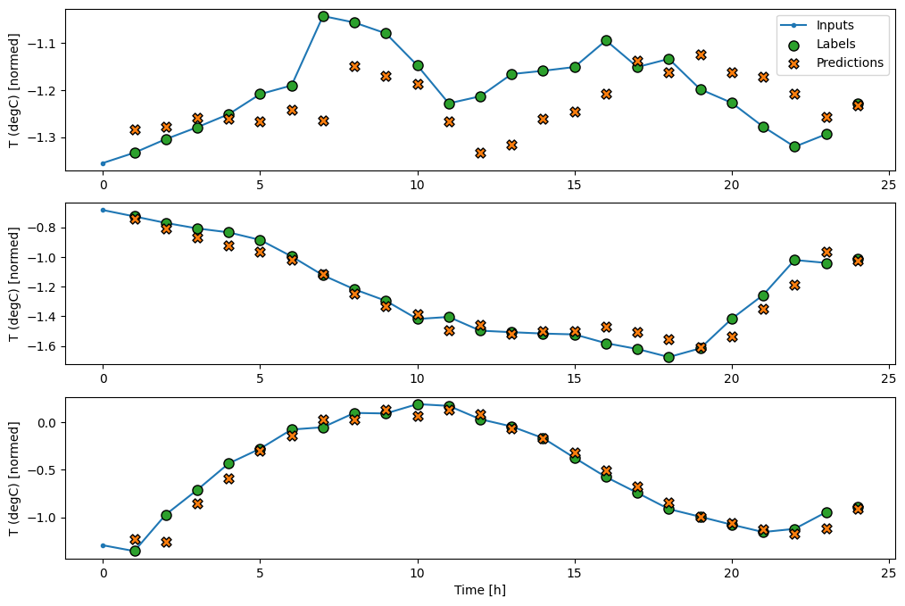
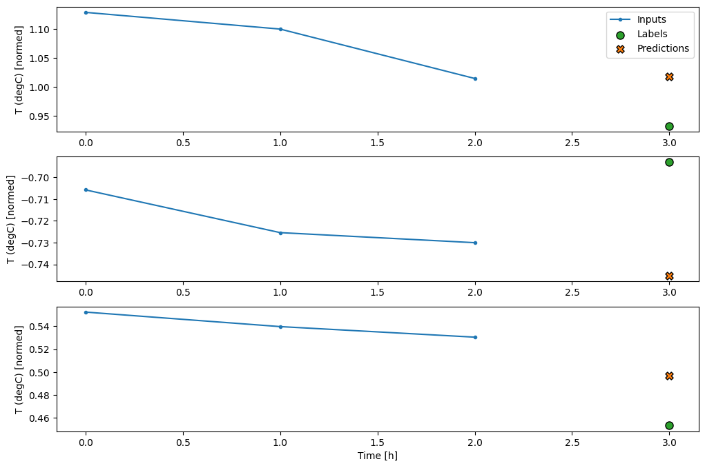
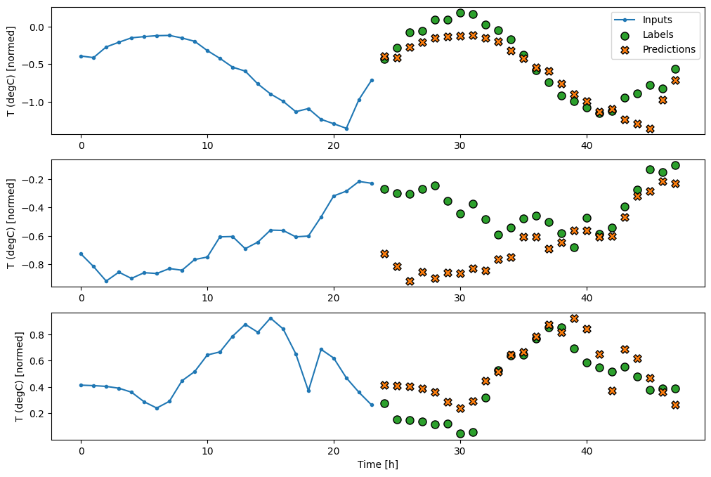
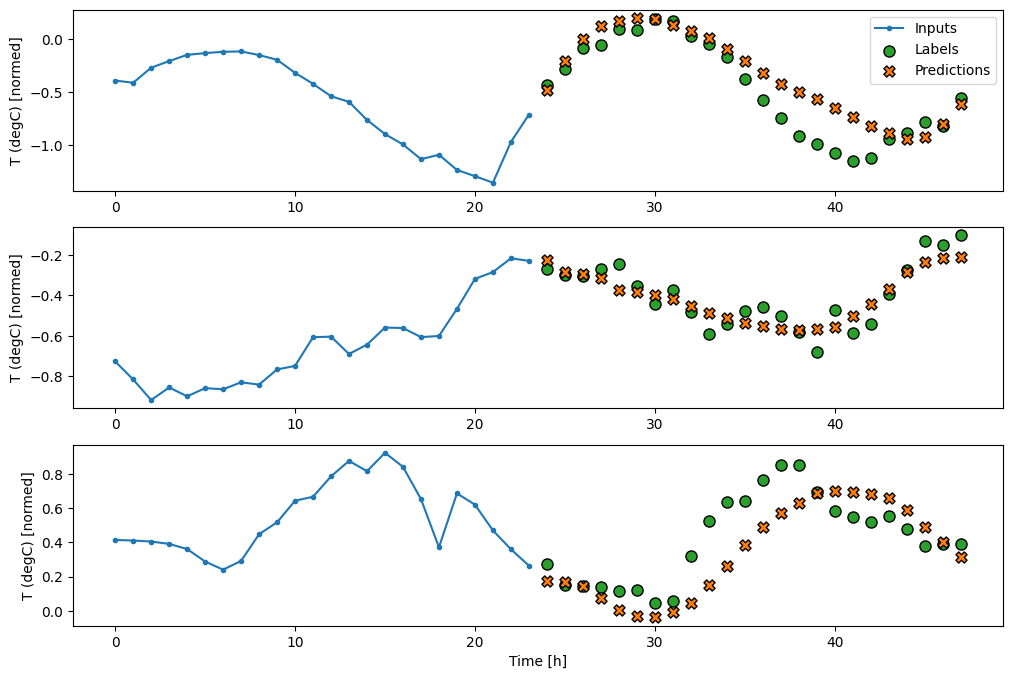
透過繪製基準模型的預測,請注意它只是標籤向右偏移一小時
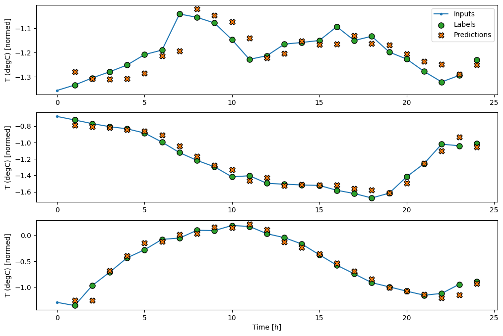
wide_window.plot(baseline)
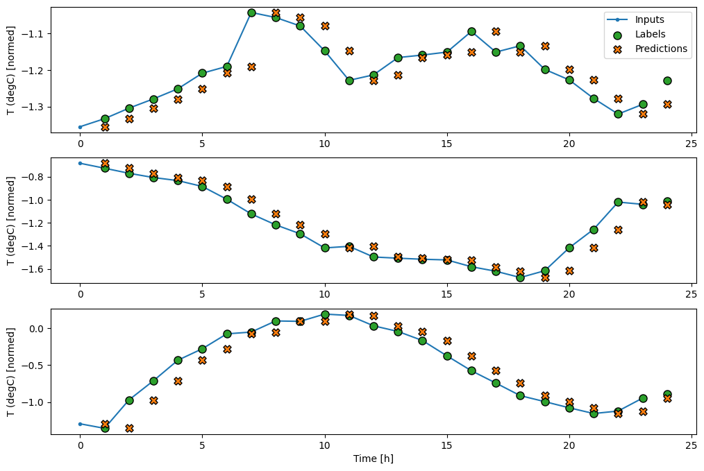
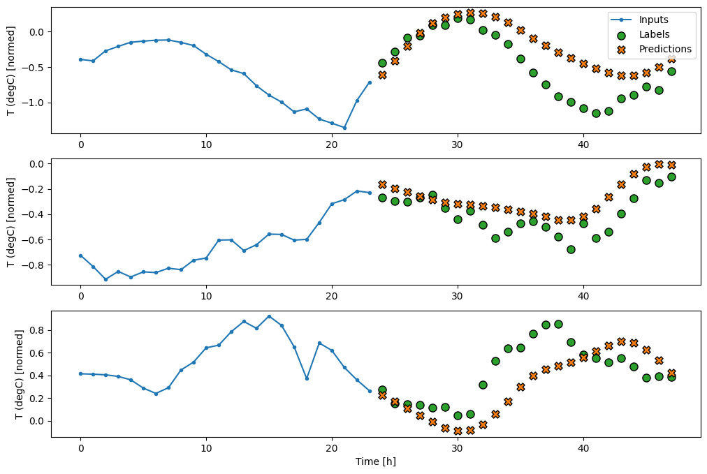
在上述三個範例的繪圖中,單一步驟模型在 24 小時的過程中執行。這值得解釋一下
- 藍色
Inputs線條顯示每個時間步的輸入溫度。模型接收所有特徵,此繪圖僅顯示溫度。 - 綠色
Labels點顯示目標預測值。這些點顯示在預測時間,而不是輸入時間。這就是為什麼標籤的範圍相對於輸入偏移 1 個步驟的原因。 - 橘色
Predictions交叉是模型針對每個輸出時間步的預測。如果模型預測完美,則預測會直接落在Labels上。
線性模型
您可以套用至此任務的最簡單可訓練模型是在輸入和輸出之間插入線性轉換。在本例中,來自時間步的輸出僅取決於該步驟
沒有設定 activation 的 tf.keras.layers.Dense 層是線性模型。該層只會將資料的最後一個軸從 (batch, time, inputs) 轉換為 (batch, time, units);它會獨立套用至 batch 和 time 軸上的每個項目。
linear = tf.keras.Sequential([
    tf.keras.layers.Dense(units=1)
])
print('Input shape:', single_step_window.example[0].shape)
print('Output shape:', linear(single_step_window.example[0]).shape)
Input shape: (32, 1, 19)
Output shape: (32, 1, 1)
本教學課程訓練許多模型,因此將訓練程序封裝到函式中
MAX_EPOCHS = 20

def compile_and_fit(model, window, patience=2):
  early_stopping = tf.keras.callbacks.EarlyStopping(monitor='val_loss',
                                                    patience=patience,
                                                    mode='min')

  model.compile(loss=tf.keras.losses.MeanSquaredError(),
                optimizer=tf.keras.optimizers.Adam(),
                metrics=[tf.keras.metrics.MeanAbsoluteError()])

  history = model.fit(window.train, epochs=MAX_EPOCHS,
                      validation_data=window.val,
                      callbacks=[early_stopping])
  return history
訓練模型並評估其效能
history = compile_and_fit(linear, single_step_window)

val_performance['Linear'] = linear.evaluate(single_step_window.val, return_dict=True)
performance['Linear'] = linear.evaluate(single_step_window.test, verbose=0, return_dict=True)
Epoch 1/20
1534/1534 ━━━━━━━━━━━━━━━━━━━━ 4s 2ms/step - loss: 0.2368 - mean_absolute_error: 0.3324 - val_loss: 0.0157 - val_mean_absolute_error: 0.0936
Epoch 2/20
1534/1534 ━━━━━━━━━━━━━━━━━━━━ 2s 2ms/step - loss: 0.0134 - mean_absolute_error: 0.0870 - val_loss: 0.0109 - val_mean_absolute_error: 0.0790
Epoch 3/20
1534/1534 ━━━━━━━━━━━━━━━━━━━━ 2s 2ms/step - loss: 0.0100 - mean_absolute_error: 0.0741 - val_loss: 0.0091 - val_mean_absolute_error: 0.0713
Epoch 4/20
1534/1534 ━━━━━━━━━━━━━━━━━━━━ 2s 2ms/step - loss: 0.0091 - mean_absolute_error: 0.0699 - val_loss: 0.0089 - val_mean_absolute_error: 0.0701
Epoch 5/20
1534/1534 ━━━━━━━━━━━━━━━━━━━━ 2s 2ms/step - loss: 0.0090 - mean_absolute_error: 0.0695 - val_loss: 0.0088 - val_mean_absolute_error: 0.0699
Epoch 6/20
1534/1534 ━━━━━━━━━━━━━━━━━━━━ 2s 2ms/step - loss: 0.0090 - mean_absolute_error: 0.0695 - val_loss: 0.0088 - val_mean_absolute_error: 0.0696
Epoch 7/20
1534/1534 ━━━━━━━━━━━━━━━━━━━━ 2s 2ms/step - loss: 0.0090 - mean_absolute_error: 0.0693 - val_loss: 0.0089 - val_mean_absolute_error: 0.0701
Epoch 8/20
1534/1534 ━━━━━━━━━━━━━━━━━━━━ 2s 2ms/step - loss: 0.0089 - mean_absolute_error: 0.0693 - val_loss: 0.0088 - val_mean_absolute_error: 0.0698
439/439 ━━━━━━━━━━━━━━━━━━━━ 1s 1ms/step - loss: 0.0088 - mean_absolute_error: 0.0697
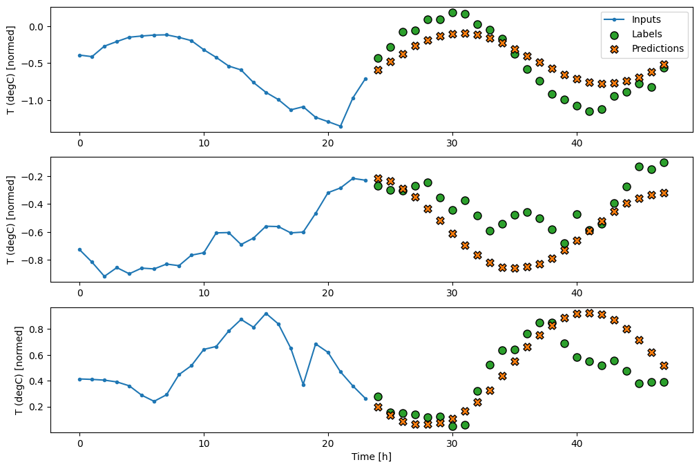
與 baseline 模型類似,線性模型可以在寬視窗批次上呼叫。以這種方式使用時,模型會對連續時間步進行一組獨立的預測。time 軸的作用就像另一個 batch 軸。每個時間步的預測之間沒有互動。
print('Input shape:', wide_window.example[0].shape)
print('Output shape:', linear(wide_window.example[0]).shape)
Input shape: (32, 24, 19)
Output shape: (32, 24, 1)
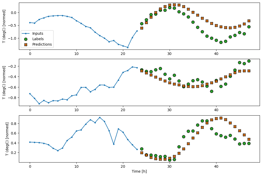
以下是其在 wide_window 上的範例預測繪圖,請注意在許多情況下,預測顯然比只傳回輸入溫度更好,但在少數情況下則更糟
wide_window.plot(linear)
線性模型的一個優點是它們相對容易解讀。您可以取出層的權重,並視覺化指派給每個輸入的權重
plt.bar(x = range(len(train_df.columns)),
        height=linear.layers[0].kernel[:,0].numpy())
axis = plt.gca()
axis.set_xticks(range(len(train_df.columns)))
_ = axis.set_xticklabels(train_df.columns, rotation=90)
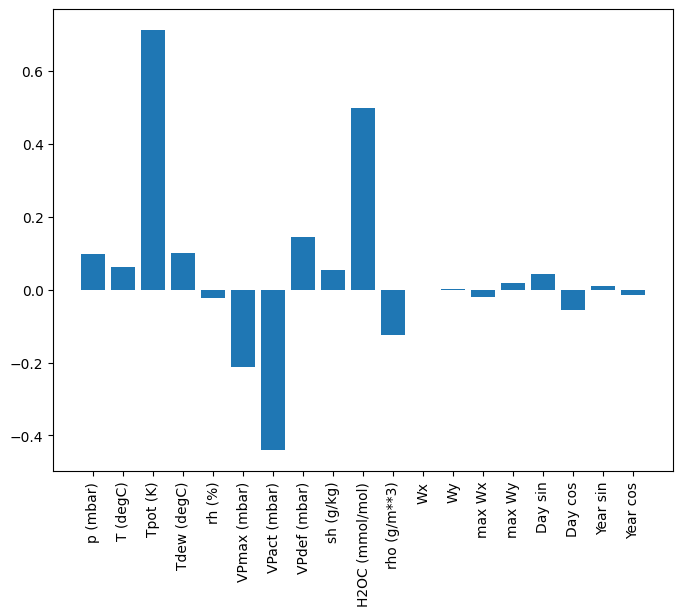
有時,模型甚至不會將最大的權重放在輸入 T (degC) 上。這是隨機初始化的風險之一。
密集
在套用實際在多個時間步上運作的模型之前,值得檢查更深層、更強大的單一輸入步驟模型的效能。
以下模型與 linear 模型類似,不同之處在於它在輸入和輸出之間堆疊了幾個 Dense 層
dense = tf.keras.Sequential([
    tf.keras.layers.Dense(units=64, activation='relu'),
    tf.keras.layers.Dense(units=64, activation='relu'),
    tf.keras.layers.Dense(units=1)
])

history = compile_and_fit(dense, single_step_window)

val_performance['Dense'] = dense.evaluate(single_step_window.val, return_dict=True)
performance['Dense'] = dense.evaluate(single_step_window.test, verbose=0, return_dict=True)
Epoch 1/20
1534/1534 ━━━━━━━━━━━━━━━━━━━━ 5s 2ms/step - loss: 0.0621 - mean_absolute_error: 0.1284 - val_loss: 0.0086 - val_mean_absolute_error: 0.0676
Epoch 2/20
1534/1534 ━━━━━━━━━━━━━━━━━━━━ 3s 2ms/step - loss: 0.0082 - mean_absolute_error: 0.0659 - val_loss: 0.0071 - val_mean_absolute_error: 0.0605
Epoch 3/20
1534/1534 ━━━━━━━━━━━━━━━━━━━━ 3s 2ms/step - loss: 0.0076 - mean_absolute_error: 0.0631 - val_loss: 0.0070 - val_mean_absolute_error: 0.0591
Epoch 4/20
1534/1534 ━━━━━━━━━━━━━━━━━━━━ 3s 2ms/step - loss: 0.0074 - mean_absolute_error: 0.0615 - val_loss: 0.0066 - val_mean_absolute_error: 0.0574
Epoch 5/20
1534/1534 ━━━━━━━━━━━━━━━━━━━━ 3s 2ms/step - loss: 0.0071 - mean_absolute_error: 0.0602 - val_loss: 0.0067 - val_mean_absolute_error: 0.0579
Epoch 6/20
1534/1534 ━━━━━━━━━━━━━━━━━━━━ 3s 2ms/step - loss: 0.0071 - mean_absolute_error: 0.0603 - val_loss: 0.0069 - val_mean_absolute_error: 0.0593
439/439 ━━━━━━━━━━━━━━━━━━━━ 1s 1ms/step - loss: 0.0072 - mean_absolute_error: 0.0601
多步驟密集
單一時間步模型沒有目前輸入值的背景資訊。它看不到輸入特徵如何隨時間變化。為了解決這個問題,模型在進行預測時需要存取多個時間步
baseline、linear 和 dense 模型獨立處理每個時間步。在這裡,模型將採用多個時間步作為輸入來產生單一輸出。
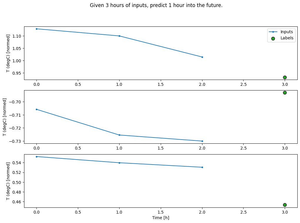
建立一個 WindowGenerator,它將產生三小時輸入和一小時標籤的批次
請注意,Window 的 shift 參數相對於兩個視窗的結尾。
CONV_WIDTH = 3
conv_window = WindowGenerator(
    input_width=CONV_WIDTH,
    label_width=1,
    shift=1,
    label_columns=['T (degC)'])

conv_window
Total window size: 4
Input indices: [0 1 2]
Label indices: [3]
Label column name(s): ['T (degC)']
conv_window.plot()
plt.suptitle("Given 3 hours of inputs, predict 1 hour into the future.")
Text(0.5, 0.98, 'Given 3 hours of inputs, predict 1 hour into the future.')
您可以透過新增 tf.keras.layers.Flatten 作為模型的第一層,來訓練多輸入步驟視窗的 dense 模型
multi_step_dense = tf.keras.Sequential([
    # Shape: (time, features) => (time*features)
    tf.keras.layers.Flatten(),
    tf.keras.layers.Dense(units=32, activation='relu'),
    tf.keras.layers.Dense(units=32, activation='relu'),
    tf.keras.layers.Dense(units=1),
    # Add back the time dimension.
    # Shape: (outputs) => (1, outputs)
    tf.keras.layers.Reshape([1, -1]),
])
print('Input shape:', conv_window.example[0].shape)
print('Output shape:', multi_step_dense(conv_window.example[0]).shape)
Input shape: (32, 3, 19)
Output shape: (32, 1, 1)
history = compile_and_fit(multi_step_dense, conv_window)

IPython.display.clear_output()
val_performance['Multi step dense'] = multi_step_dense.evaluate(conv_window.val, return_dict=True)
performance['Multi step dense'] = multi_step_dense.evaluate(conv_window.test, verbose=0, return_dict=True)
438/438 ━━━━━━━━━━━━━━━━━━━━ 1s 1ms/step - loss: 0.0067 - mean_absolute_error: 0.0590
conv_window.plot(multi_step_dense)
這種方法的主要缺點是,產生的模型只能在形狀完全相同的輸入視窗上執行。
print('Input shape:', wide_window.example[0].shape)
try:
  print('Output shape:', multi_step_dense(wide_window.example[0]).shape)
except Exception as e:
  print(f'\n{type(e).__name__}:{e}')
Input shape: (32, 24, 19)

ValueError:Exception encountered when calling Sequential.call().

Input 0 of layer "dense_4" is incompatible with the layer: expected axis -1 of input shape to have value 57, but received input with shape (32, 456)

Arguments received by Sequential.call():
  • inputs=tf.Tensor(shape=(32, 24, 19), dtype=float32)
  • training=None
  • mask=None
下一節中的卷積模型修正了這個問題。
卷積神經網路
卷積層 (tf.keras.layers.Conv1D) 也會採用多個時間步作為每個預測的輸入。
以下是與 multi_step_dense 相同的模型,以卷積重新撰寫。
請注意變更
tf.keras.layers.Flatten和第一個tf.keras.layers.Dense由tf.keras.layers.Conv1D取代。- 由於卷積會在輸出中保留時間軸,因此不再需要
tf.keras.layers.Reshape。
conv_model = tf.keras.Sequential([
    tf.keras.layers.Conv1D(filters=32,
                           kernel_size=(CONV_WIDTH,),
                           activation='relu'),
    tf.keras.layers.Dense(units=32, activation='relu'),
    tf.keras.layers.Dense(units=1),
])
在範例批次上執行它,以檢查模型是否產生具有預期形狀的輸出
print("Conv model on `conv_window`")
print('Input shape:', conv_window.example[0].shape)
print('Output shape:', conv_model(conv_window.example[0]).shape)
Conv model on `conv_window`
Input shape: (32, 3, 19)
Output shape: (32, 1, 1)
在 conv_window 上訓練和評估它,它應該提供與 multi_step_dense 模型類似的效能。
history = compile_and_fit(conv_model, conv_window)

IPython.display.clear_output()
val_performance['Conv'] = conv_model.evaluate(conv_window.val, return_dict=True)
performance['Conv'] = conv_model.evaluate(conv_window.test, verbose=0, return_dict=True)
438/438 ━━━━━━━━━━━━━━━━━━━━ 1s 1ms/step - loss: 0.0075 - mean_absolute_error: 0.0615
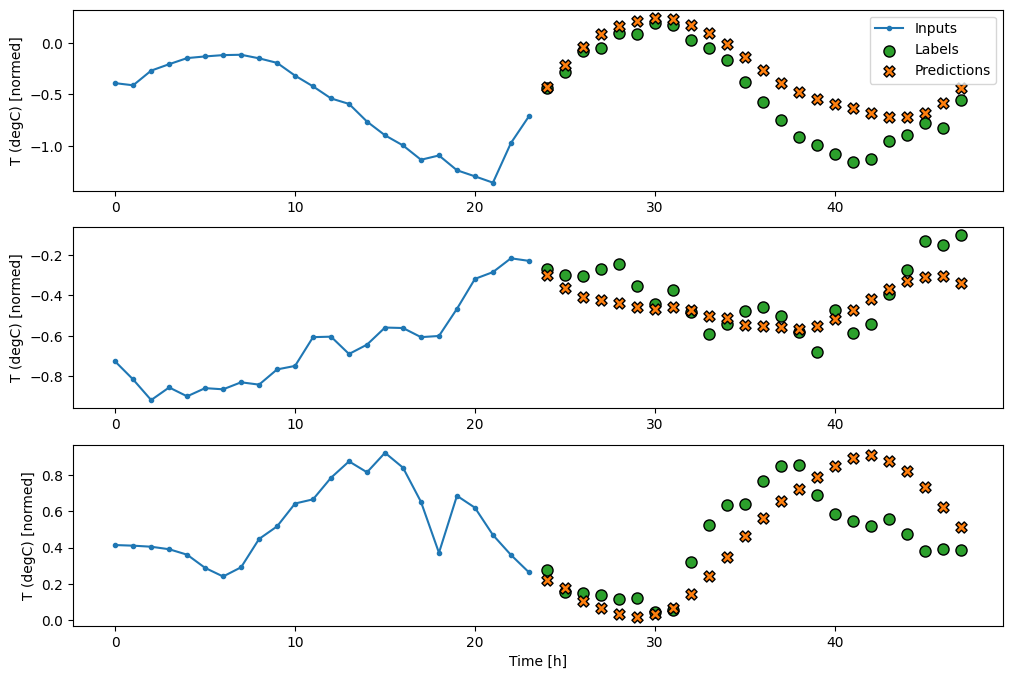
此 conv_model 與 multi_step_dense 模型之間的差異在於 conv_model 可以針對任何長度的輸入執行。卷積層會套用至輸入的滑動視窗
如果您在更寬的輸入上執行它,它會產生更寬的輸出
print("Wide window")
print('Input shape:', wide_window.example[0].shape)
print('Labels shape:', wide_window.example[1].shape)
print('Output shape:', conv_model(wide_window.example[0]).shape)
Wide window
Input shape: (32, 24, 19)
Labels shape: (32, 24, 1)
Output shape: (32, 22, 1)
請注意,輸出比輸入短。為了使訓練或繪圖工作正常運作,您需要標籤和預測具有相同的長度。因此,請建立一個 WindowGenerator,以產生具有一些額外輸入時間步的寬視窗,以便標籤和預測長度相符
LABEL_WIDTH = 24
INPUT_WIDTH = LABEL_WIDTH + (CONV_WIDTH - 1)
wide_conv_window = WindowGenerator(
    input_width=INPUT_WIDTH,
    label_width=LABEL_WIDTH,
    shift=1,
    label_columns=['T (degC)'])

wide_conv_window
Total window size: 27
Input indices: [ 0  1  2  3  4  5  6  7  8  9 10 11 12 13 14 15 16 17 18 19 20 21 22 23
 24 25]
Label indices: [ 3  4  5  6  7  8  9 10 11 12 13 14 15 16 17 18 19 20 21 22 23 24 25 26]
Label column name(s): ['T (degC)']
print("Wide conv window")
print('Input shape:', wide_conv_window.example[0].shape)
print('Labels shape:', wide_conv_window.example[1].shape)
print('Output shape:', conv_model(wide_conv_window.example[0]).shape)
Wide conv window
Input shape: (32, 26, 19)
Labels shape: (32, 24, 1)
Output shape: (32, 24, 1)
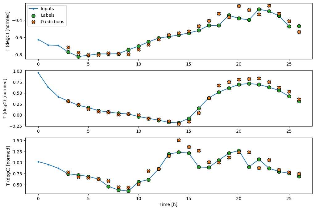
現在,您可以在更寬的視窗上繪製模型的預測。請注意第一個預測之前的 3 個輸入時間步。這裡的每個預測都基於前 3 個時間步
wide_conv_window.plot(conv_model)
循環神經網路
循環神經網路 (RNN) 是一種非常適合時間序列資料的神經網路。RNN 會逐步處理時間序列,並在每個時間步之間維護內部狀態。
您可以在「使用 RNN 進行文字生成」教學課程和「使用 Keras 的循環神經網路 (RNN)」指南中了解更多資訊。
在本教學課程中,您將使用一個名為長短期記憶 (LSTM) 的 RNN 層 (tf.keras.layers.LSTM)。
對於所有 Keras RNN 層 (例如 tf.keras.layers.LSTM) 而言,一個重要的建構子引數是 return_sequences 引數。此設定可以用兩種方式設定層
- 如果
False(預設值),則該層只會傳回最後一個時間步的輸出,讓模型有時間預熱其內部狀態,然後再進行單一預測
- 如果
True,則該層會為每個輸入傳回一個輸出。這對於以下情況很有用:- 堆疊 RNN 層。
- 同時在多個時間步上訓練模型。
lstm_model = tf.keras.models.Sequential([
    # Shape [batch, time, features] => [batch, time, lstm_units]
    tf.keras.layers.LSTM(32, return_sequences=True),
    # Shape => [batch, time, features]
    tf.keras.layers.Dense(units=1)
])
使用 return_sequences=True,模型可以一次在 24 小時的資料上進行訓練。
print('Input shape:', wide_window.example[0].shape)
print('Output shape:', lstm_model(wide_window.example[0]).shape)
Input shape: (32, 24, 19)
Output shape: (32, 24, 1)
history = compile_and_fit(lstm_model, wide_window)

IPython.display.clear_output()
val_performance['LSTM'] = lstm_model.evaluate(wide_window.val, return_dict=True)
performance['LSTM'] = lstm_model.evaluate(wide_window.test, verbose=0, return_dict=True)
438/438 ━━━━━━━━━━━━━━━━━━━━ 1s 2ms/step - loss: 0.0055 - mean_absolute_error: 0.0511
wide_window.plot(lstm_model)
效能
使用此資料集,通常每個模型的效能都比前一個模型稍微好一點。
cm = lstm_model.metrics[1]
cm.metrics
[<MeanAbsoluteError name=mean_absolute_error>]
val_performance
{'Baseline': {'loss': 0.012845639139413834,
  'mean_absolute_error': 0.0784662663936615},
 'Linear': {'loss': 0.00884665921330452,
  'mean_absolute_error': 0.0698472261428833},
 'Dense': {'loss': 0.006883115507662296,
  'mean_absolute_error': 0.05929134413599968},
 'Multi step dense': {'loss': 0.006829570047557354,
  'mean_absolute_error': 0.05932893231511116},
 'Conv': {'loss': 0.007479575928300619,
  'mean_absolute_error': 0.06144466996192932},
 'LSTM': {'loss': 0.005511085502803326,
  'mean_absolute_error': 0.050988875329494476} }
x = np.arange(len(performance))
width = 0.3
metric_name = 'mean_absolute_error'
val_mae = [v[metric_name] for v in val_performance.values()]
test_mae = [v[metric_name] for v in performance.values()]

plt.ylabel('mean_absolute_error [T (degC), normalized]')
plt.bar(x - 0.17, val_mae, width, label='Validation')
plt.bar(x + 0.17, test_mae, width, label='Test')
plt.xticks(ticks=x, labels=performance.keys(),
           rotation=45)
_ = plt.legend()
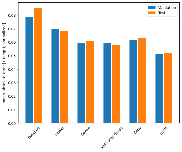
for name, value in performance.items():
  print(f'{name:12s}: {value[metric_name]:0.4f}')
Baseline    : 0.0852
Linear      : 0.0683
Dense       : 0.0611
Multi step dense: 0.0582
Conv        : 0.0629
LSTM        : 0.0520
多輸出模型
到目前為止,所有模型都預測單一輸出特徵 T (degC),針對單一時間步。
只要變更輸出層中的單元數,並調整訓練視窗以包含 labels (example_labels) 中的所有特徵,所有這些模型都可以轉換為預測多個特徵。
single_step_window = WindowGenerator(
    # `WindowGenerator` returns all features as labels if you
    # don't set the `label_columns` argument.
    input_width=1, label_width=1, shift=1)

wide_window = WindowGenerator(
    input_width=24, label_width=24, shift=1)

for example_inputs, example_labels in wide_window.train.take(1):
  print(f'Inputs shape (batch, time, features): {example_inputs.shape}')
  print(f'Labels shape (batch, time, features): {example_labels.shape}')
Inputs shape (batch, time, features): (32, 24, 19)
Labels shape (batch, time, features): (32, 24, 19)
2024-06-30 02:54:37.053087: W tensorflow/core/framework/local_rendezvous.cc:404] Local rendezvous is aborting with status: OUT_OF_RANGE: End of sequence
請注意,標籤的 features 軸現在具有與輸入相同的深度,而不是 1。
基準
此處可以使用相同的基準模型 (Baseline),但這次是重複所有特徵,而不是選取特定的 label_index。
baseline = Baseline()
baseline.compile(loss=tf.keras.losses.MeanSquaredError(),
                 metrics=[tf.keras.metrics.MeanAbsoluteError()])
val_performance = {}
performance = {}
val_performance['Baseline'] = baseline.evaluate(wide_window.val, return_dict=True)
performance['Baseline'] = baseline.evaluate(wide_window.test, verbose=0, return_dict=True)
438/438 ━━━━━━━━━━━━━━━━━━━━ 1s 1ms/step - loss: 0.0885 - mean_absolute_error: 0.1588
密集
dense = tf.keras.Sequential([
    tf.keras.layers.Dense(units=64, activation='relu'),
    tf.keras.layers.Dense(units=64, activation='relu'),
    tf.keras.layers.Dense(units=num_features)
])
history = compile_and_fit(dense, single_step_window)

IPython.display.clear_output()
val_performance['Dense'] = dense.evaluate(single_step_window.val, return_dict=True)
performance['Dense'] = dense.evaluate(single_step_window.test, verbose=0, return_dict=True)
439/439 ━━━━━━━━━━━━━━━━━━━━ 1s 1ms/step - loss: 0.0665 - mean_absolute_error: 0.1280
RNN
%%time
wide_window = WindowGenerator(
    input_width=24, label_width=24, shift=1)

lstm_model = tf.keras.models.Sequential([
    # Shape [batch, time, features] => [batch, time, lstm_units]
    tf.keras.layers.LSTM(32, return_sequences=True),
    # Shape => [batch, time, features]
    tf.keras.layers.Dense(units=num_features)
])

history = compile_and_fit(lstm_model, wide_window)

IPython.display.clear_output()
val_performance['LSTM'] = lstm_model.evaluate( wide_window.val, return_dict=True)
performance['LSTM'] = lstm_model.evaluate( wide_window.test, verbose=0, return_dict=True)

print()
438/438 ━━━━━━━━━━━━━━━━━━━━ 1s 2ms/step - loss: 0.0614 - mean_absolute_error: 0.1205

CPU times: user 4min 8s, sys: 48.8 s, total: 4min 57s
Wall time: 1min 48s
進階:殘差連接
先前的 Baseline 模型利用了序列從一個時間步到另一個時間步之間不會劇烈變動的事實。到目前為止,本教學課程中訓練的每個模型都是隨機初始化的,然後必須學習輸出是與前一個時間步的小幅變動。
雖然您可以透過謹慎的初始化來解決這個問題,但將其建置到模型結構中會更簡單。
在時間序列分析中,常見的做法是建置模型,以預測值在下一個時間步中將如何變化,而不是預測下一個值。同樣地,深度學習中的殘差網路(或 ResNet)指的是每個層都會新增到模型的累積結果中的架構。
這就是您如何利用變動應該很小的知識。
基本上,這會初始化模型以符合 Baseline。對於此任務,它有助於模型更快收斂,並具有稍微好一點的效能。
這種方法可以與本教學課程中討論的任何模型結合使用。
在此,它正應用於 LSTM 模型,請注意使用 tf.initializers.zeros 以確保初始預測變動很小,且不會壓過殘差連接。此處的梯度沒有對稱性破壞問題,因為 zeros 只在最後一層使用。
class ResidualWrapper(tf.keras.Model):
  def __init__(self, model):
    super().__init__()
    self.model = model

  def call(self, inputs, *args, **kwargs):
    delta = self.model(inputs, *args, **kwargs)

    # The prediction for each time step is the input
    # from the previous time step plus the delta
    # calculated by the model.
    return inputs + delta
%%time
residual_lstm = ResidualWrapper(
    tf.keras.Sequential([
    tf.keras.layers.LSTM(32, return_sequences=True),
    tf.keras.layers.Dense(
        num_features,
        # The predicted deltas should start small.
        # Therefore, initialize the output layer with zeros.
        kernel_initializer=tf.initializers.zeros())
]))

history = compile_and_fit(residual_lstm, wide_window)

IPython.display.clear_output()
val_performance['Residual LSTM'] = residual_lstm.evaluate(wide_window.val, return_dict=True)
performance['Residual LSTM'] = residual_lstm.evaluate(wide_window.test, verbose=0, return_dict=True)
print()
438/438 ━━━━━━━━━━━━━━━━━━━━ 1s 2ms/step - loss: 0.0619 - mean_absolute_error: 0.1179

CPU times: user 1min 51s, sys: 22.2 s, total: 2min 13s
Wall time: 49.4 s
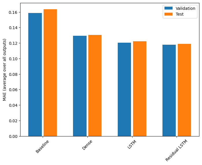
效能
以下是這些多輸出模型的整體效能。
x = np.arange(len(performance))
width = 0.3

metric_name = 'mean_absolute_error'
val_mae = [v[metric_name] for v in val_performance.values()]
test_mae = [v[metric_name] for v in performance.values()]

plt.bar(x - 0.17, val_mae, width, label='Validation')
plt.bar(x + 0.17, test_mae, width, label='Test')
plt.xticks(ticks=x, labels=performance.keys(),
           rotation=45)
plt.ylabel('MAE (average over all outputs)')
_ = plt.legend()
for name, value in performance.items():
  print(f'{name:15s}: {value[metric_name]:0.4f}')
Baseline       : 0.1638
Dense          : 0.1307
LSTM           : 0.1223
Residual LSTM  : 0.1191
上述效能是在所有模型輸出之間平均得出的。
多步模型
先前章節中的單輸出和多輸出模型都進行了單一時間步預測,預測未來一小時。
本節探討如何擴展這些模型以進行多時間步預測。
在多步預測中,模型需要學習預測一系列未來值。因此,與僅預測單一未來點的單步模型不同,多步模型會預測一系列未來值。
對此有兩種粗略方法
- 一次性預測,其中整個時間序列一次預測完成。
- 自迴歸預測,其中模型僅進行單步預測,且其輸出會作為其輸入回饋。
在本節中,所有模型都將預測跨所有輸出時間步的所有特徵。
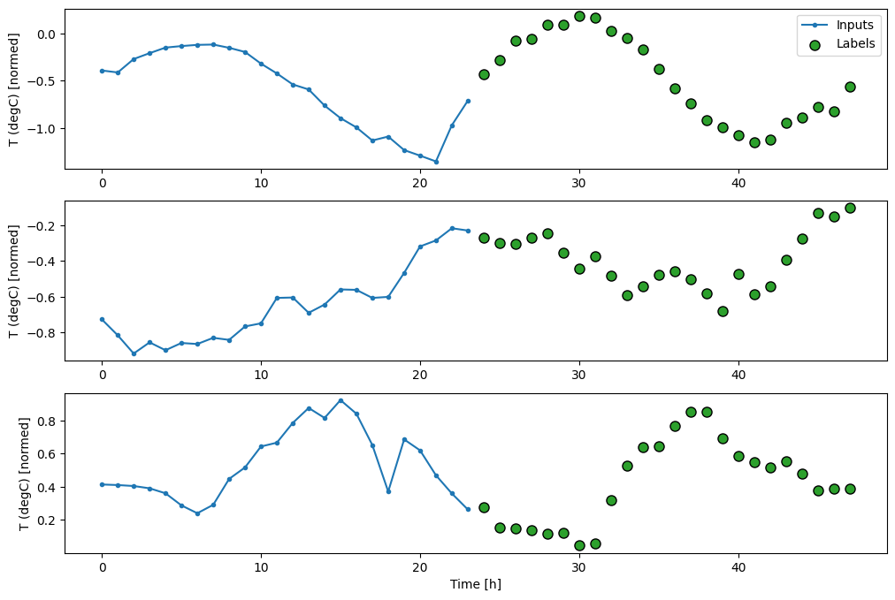
對於多步模型,訓練資料再次包含每小時樣本。但是,在此,模型將學習預測未來 24 小時,給定過去 24 小時的資料。
以下是一個 Window 物件,可從資料集中產生這些切片
OUT_STEPS = 24
multi_window = WindowGenerator(input_width=24,
                               label_width=OUT_STEPS,
                               shift=OUT_STEPS)

multi_window.plot()
multi_window
Total window size: 48
Input indices: [ 0  1  2  3  4  5  6  7  8  9 10 11 12 13 14 15 16 17 18 19 20 21 22 23]
Label indices: [24 25 26 27 28 29 30 31 32 33 34 35 36 37 38 39 40 41 42 43 44 45 46 47]
Label column name(s): None
基準
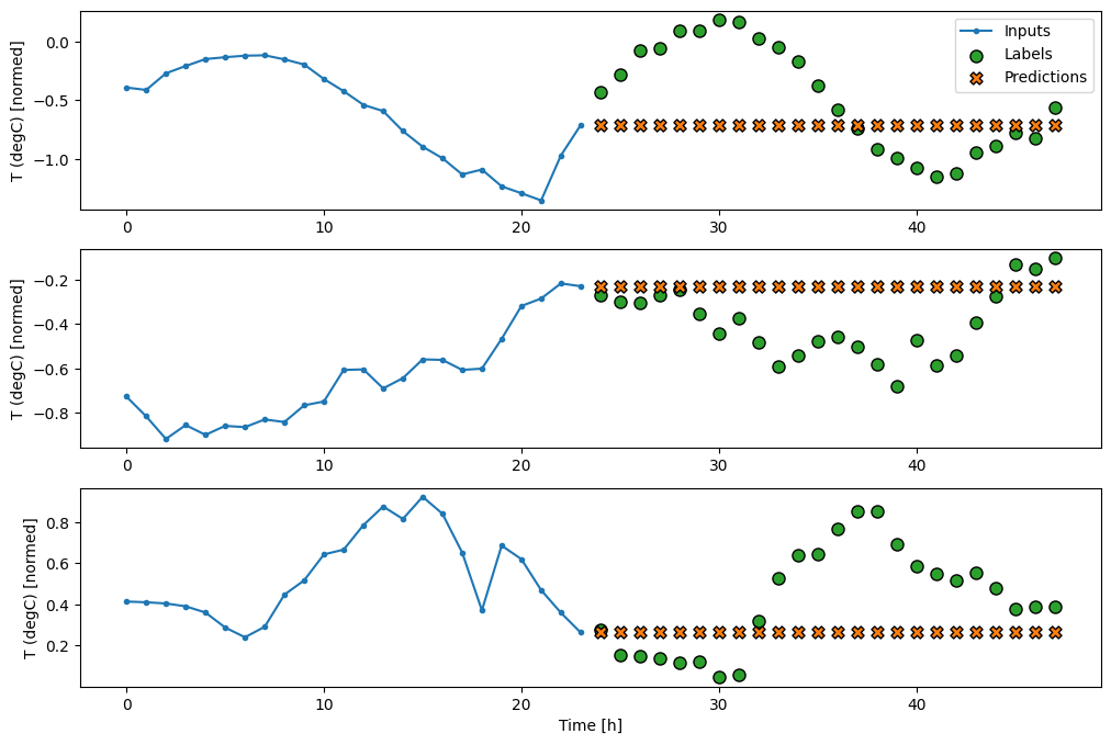
此任務的一個簡單基準是重複最後一個輸入時間步,以達到所需的輸出時間步數。
class MultiStepLastBaseline(tf.keras.Model):
  def call(self, inputs):
    return tf.tile(inputs[:, -1:, :], [1, OUT_STEPS, 1])

last_baseline = MultiStepLastBaseline()
last_baseline.compile(loss=tf.keras.losses.MeanSquaredError(),
                      metrics=[tf.keras.metrics.MeanAbsoluteError()])

multi_val_performance = {}
multi_performance = {}

multi_val_performance['Last'] = last_baseline.evaluate(multi_window.val, return_dict=True)
multi_performance['Last'] = last_baseline.evaluate(multi_window.test, verbose=0, return_dict=True)
multi_window.plot(last_baseline)
437/437 ━━━━━━━━━━━━━━━━━━━━ 1s 2ms/step - loss: 0.6305 - mean_absolute_error: 0.5020
由於此任務是預測未來 24 小時,給定過去 24 小時的資料,因此另一種簡單的方法是重複前一天,假設明天會相似。
class RepeatBaseline(tf.keras.Model):
  def call(self, inputs):
    return inputs

repeat_baseline = RepeatBaseline()
repeat_baseline.compile(loss=tf.keras.losses.MeanSquaredError(),
                        metrics=[tf.keras.metrics.MeanAbsoluteError()])

multi_val_performance['Repeat'] = repeat_baseline.evaluate(multi_window.val, return_dict=True)
multi_performance['Repeat'] = repeat_baseline.evaluate(multi_window.test, verbose=0, return_dict=True)
multi_window.plot(repeat_baseline)
437/437 ━━━━━━━━━━━━━━━━━━━━ 1s 1ms/step - loss: 0.4276 - mean_absolute_error: 0.3954
一次性模型
針對此問題的一種高階方法是使用「一次性」模型,其中模型在單一步驟中完成整個序列預測。
這可以有效率地實作為具有 OUT_STEPS*features 輸出單元的 tf.keras.layers.Dense。模型只需要將該輸出重塑為所需的 (OUTPUT_STEPS, features)。
線性
基於最後一個輸入時間步的簡單線性模型比任何一個基準都好,但功能不足。模型需要從具有線性投影的單一輸入時間步預測 OUTPUT_STEPS 時間步。它只能捕捉行為的低維度切片,可能主要基於一天中的時間和一年中的時間。

multi_linear_model = tf.keras.Sequential([
    # Take the last time-step.
    # Shape [batch, time, features] => [batch, 1, features]
    tf.keras.layers.Lambda(lambda x: x[:, -1:, :]),
    # Shape => [batch, 1, out_steps*features]
    tf.keras.layers.Dense(OUT_STEPS*num_features,
                          kernel_initializer=tf.initializers.zeros()),
    # Shape => [batch, out_steps, features]
    tf.keras.layers.Reshape([OUT_STEPS, num_features])
])

history = compile_and_fit(multi_linear_model, multi_window)

IPython.display.clear_output()
multi_val_performance['Linear'] = multi_linear_model.evaluate(multi_window.val, return_dict=True)
multi_performance['Linear'] = multi_linear_model.evaluate(multi_window.test, verbose=0, return_dict=True)
multi_window.plot(multi_linear_model)
437/437 ━━━━━━━━━━━━━━━━━━━━ 1s 1ms/step - loss: 0.2523 - mean_absolute_error: 0.3035
密集
在輸入和輸出之間新增 tf.keras.layers.Dense 可為線性模型提供更多功能,但仍然僅基於單一輸入時間步。
multi_dense_model = tf.keras.Sequential([
    # Take the last time step.
    # Shape [batch, time, features] => [batch, 1, features]
    tf.keras.layers.Lambda(lambda x: x[:, -1:, :]),
    # Shape => [batch, 1, dense_units]
    tf.keras.layers.Dense(512, activation='relu'),
    # Shape => [batch, out_steps*features]
    tf.keras.layers.Dense(OUT_STEPS*num_features,
                          kernel_initializer=tf.initializers.zeros()),
    # Shape => [batch, out_steps, features]
    tf.keras.layers.Reshape([OUT_STEPS, num_features])
])

history = compile_and_fit(multi_dense_model, multi_window)

IPython.display.clear_output()
multi_val_performance['Dense'] = multi_dense_model.evaluate(multi_window.val, return_dict=True)
multi_performance['Dense'] = multi_dense_model.evaluate(multi_window.test, verbose=0, return_dict=True)
multi_window.plot(multi_dense_model)
437/437 ━━━━━━━━━━━━━━━━━━━━ 1s 1ms/step - loss: 0.2158 - mean_absolute_error: 0.2793
CNN
卷積模型根據固定寬度歷史記錄進行預測,這可能會比密集模型帶來更好的效能,因為它可以查看事物如何隨時間變化。
CONV_WIDTH = 3
multi_conv_model = tf.keras.Sequential([
    # Shape [batch, time, features] => [batch, CONV_WIDTH, features]
    tf.keras.layers.Lambda(lambda x: x[:, -CONV_WIDTH:, :]),
    # Shape => [batch, 1, conv_units]
    tf.keras.layers.Conv1D(256, activation='relu', kernel_size=(CONV_WIDTH)),
    # Shape => [batch, 1,  out_steps*features]
    tf.keras.layers.Dense(OUT_STEPS*num_features,
                          kernel_initializer=tf.initializers.zeros()),
    # Shape => [batch, out_steps, features]
    tf.keras.layers.Reshape([OUT_STEPS, num_features])
])

history = compile_and_fit(multi_conv_model, multi_window)

IPython.display.clear_output()

multi_val_performance['Conv'] = multi_conv_model.evaluate(multi_window.val, return_dict=True)
multi_performance['Conv'] = multi_conv_model.evaluate(multi_window.test, verbose=0, return_dict=True)
multi_window.plot(multi_conv_model)
437/437 ━━━━━━━━━━━━━━━━━━━━ 1s 1ms/step - loss: 0.2154 - mean_absolute_error: 0.2798
RNN
如果循環模型與模型正在進行的預測相關,則循環模型可以學習使用長時間的輸入歷史記錄。在此,模型將累積 24 小時的內部狀態,然後再針對未來 24 小時進行單一預測。
在此一次性格式中,LSTM 只需要在最後一個時間步產生輸出,因此請在 tf.keras.layers.LSTM 中設定 return_sequences=False。
multi_lstm_model = tf.keras.Sequential([
    # Shape [batch, time, features] => [batch, lstm_units].
    # Adding more `lstm_units` just overfits more quickly.
    tf.keras.layers.LSTM(32, return_sequences=False),
    # Shape => [batch, out_steps*features].
    tf.keras.layers.Dense(OUT_STEPS*num_features,
                          kernel_initializer=tf.initializers.zeros()),
    # Shape => [batch, out_steps, features].
    tf.keras.layers.Reshape([OUT_STEPS, num_features])
])

history = compile_and_fit(multi_lstm_model, multi_window)

IPython.display.clear_output()

multi_val_performance['LSTM'] = multi_lstm_model.evaluate(multi_window.val, return_dict=True)
multi_performance['LSTM'] = multi_lstm_model.evaluate(multi_window.test, verbose=0, return_dict=True)
multi_window.plot(multi_lstm_model)
437/437 ━━━━━━━━━━━━━━━━━━━━ 1s 2ms/step - loss: 0.2132 - mean_absolute_error: 0.2829
進階:自迴歸模型
上述模型都在單一步驟中預測整個輸出序列。
在某些情況下,模型將此預測分解為個別時間步可能很有幫助。然後,每個模型的輸出可以在每個步驟回饋到自身,並且可以根據先前的預測進行預測,就像經典的使用循環神經網路產生序列中一樣。
這種模型風格的一個明顯優勢是,它可以設定為產生具有變動長度的輸出。
您可以採用本教學課程前半部分中訓練的任何單步多輸出模型,並在自迴歸回饋迴圈中執行,但在此您將專注於建置一個經過明確訓練以執行此操作的模型。
RNN
本教學課程僅建置自迴歸 RNN 模型,但此模式可以應用於任何設計為輸出單一時間步的模型。
模型將具有與先前的單步 LSTM 模型相同的基本形式:一個 tf.keras.layers.LSTM 層,後跟一個 tf.keras.layers.Dense 層,該層會將 LSTM 層的輸出轉換為模型預測。
tf.keras.layers.LSTM 是一個 tf.keras.layers.LSTMCell,包裝在更高層級的 tf.keras.layers.RNN 中,後者會為您管理狀態和序列結果(請查看使用 Keras 的循環神經網路 (RNN)指南以了解詳細資訊)。
在這種情況下,模型必須手動管理每個步驟的輸入,因此它直接使用 tf.keras.layers.LSTMCell 作為更低層級的單一時間步介面。
class FeedBack(tf.keras.Model):
  def __init__(self, units, out_steps):
    super().__init__()
    self.out_steps = out_steps
    self.units = units
    self.lstm_cell = tf.keras.layers.LSTMCell(units)
    # Also wrap the LSTMCell in an RNN to simplify the `warmup` method.
    self.lstm_rnn = tf.keras.layers.RNN(self.lstm_cell, return_state=True)
    self.dense = tf.keras.layers.Dense(num_features)
feedback_model = FeedBack(units=32, out_steps=OUT_STEPS)
此模型需要的第一個方法是 warmup 方法,以根據輸入初始化其內部狀態。經過訓練後,此狀態將捕捉輸入歷史記錄的相關部分。這等同於先前的單步 LSTM 模型。
def warmup(self, inputs):
  # inputs.shape => (batch, time, features)
  # x.shape => (batch, lstm_units)
  x, *state = self.lstm_rnn(inputs)

  # predictions.shape => (batch, features)
  prediction = self.dense(x)
  return prediction, state

FeedBack.warmup = warmup
此方法會傳回單一時間步預測和 LSTM 的內部狀態。
prediction, state = feedback_model.warmup(multi_window.example[0])
prediction.shape
TensorShape([32, 19])
透過 RNN 的狀態和初始預測,您現在可以繼續迭代模型,在每個步驟回饋預測作為輸入。
收集輸出預測的最簡單方法是使用 Python 列表和迴圈後的 tf.stack。
def call(self, inputs, training=None):
  # Use a TensorArray to capture dynamically unrolled outputs.
  predictions = []
  # Initialize the LSTM state.
  prediction, state = self.warmup(inputs)

  # Insert the first prediction.
  predictions.append(prediction)

  # Run the rest of the prediction steps.
  for n in range(1, self.out_steps):
    # Use the last prediction as input.
    x = prediction
    # Execute one lstm step.
    x, state = self.lstm_cell(x, states=state,
                              training=training)
    # Convert the lstm output to a prediction.
    prediction = self.dense(x)
    # Add the prediction to the output.
    predictions.append(prediction)

  # predictions.shape => (time, batch, features)
  predictions = tf.stack(predictions)
  # predictions.shape => (batch, time, features)
  predictions = tf.transpose(predictions, [1, 0, 2])
  return predictions

FeedBack.call = call
在範例輸入上測試執行此模型
print('Output shape (batch, time, features): ', feedback_model(multi_window.example[0]).shape)
Output shape (batch, time, features): (32, 24, 19)
現在,訓練模型
history = compile_and_fit(feedback_model, multi_window)

IPython.display.clear_output()

multi_val_performance['AR LSTM'] = feedback_model.evaluate(multi_window.val, return_dict=True)
multi_performance['AR LSTM'] = feedback_model.evaluate(multi_window.test, verbose=0, return_dict=True)
multi_window.plot(feedback_model)
437/437 ━━━━━━━━━━━━━━━━━━━━ 1s 2ms/step - loss: 0.2277 - mean_absolute_error: 0.3026
效能
在這個問題上,模型複雜度的函數顯然存在邊際效益遞減。
x = np.arange(len(multi_performance))
width = 0.3

metric_name = 'mean_absolute_error'
val_mae = [v[metric_name] for v in multi_val_performance.values()]
test_mae = [v[metric_name] for v in multi_performance.values()]

plt.bar(x - 0.17, val_mae, width, label='Validation')
plt.bar(x + 0.17, test_mae, width, label='Test')
plt.xticks(ticks=x, labels=multi_performance.keys(),
           rotation=45)
plt.ylabel(f'MAE (average over all times and outputs)')
_ = plt.legend()
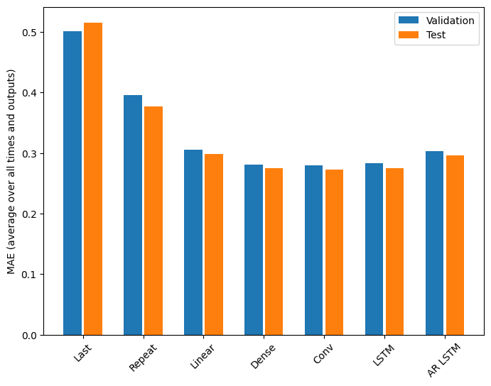
本教學課程前半部分中多輸出模型的指標顯示了在所有輸出特徵之間平均得出的效能。這些效能相似,但也是在輸出時間步之間平均得出的。
for name, value in multi_performance.items():
  print(f'{name:8s}: {value[metric_name]:0.4f}')
Last    : 0.5157
Repeat  : 0.3774
Linear  : 0.2984
Dense   : 0.2754
Conv    : 0.2723
LSTM    : 0.2745
AR LSTM : 0.2958
從密集模型轉向卷積和循環模型所獲得的增益僅為幾個百分比(如果有的話),並且自迴歸模型的效能明顯更差。因此,這些更複雜的方法可能不在這個問題上值得,但沒有嘗試就無法知道,而這些模型可能對您的問題有幫助。
後續步驟
本教學課程是使用 TensorFlow 進行時間序列預測的快速簡介。
若要了解更多資訊,請參閱
- Hands-on Machine Learning with Scikit-Learn, Keras, and TensorFlow,第 2 版的第 15 章。
- Deep Learning with Python的第 6 章。
- Udacity 的深度學習 TensorFlow 簡介的第 8 課,包括練習筆記本。
此外,請記住,您可以在 TensorFlow 中實作任何傳統時間序列模型—本教學課程僅著重於 TensorFlow 的內建功能。