基本分類：服裝圖片分類

在 TensorFlow.org 上檢視

在 Google Colab 中執行

在 GitHub 上檢視原始碼

下載筆記本

本指南訓練神經網路模型來分類服裝圖片，例如運動鞋和襯衫。如果您不瞭解所有細節也沒關係；這是快速瀏覽完整的 TensorFlow 程式，詳細資訊會在過程中逐步說明。

本指南使用 tf.keras，這是一種高階 API，可在 TensorFlow 中建構和訓練模型。

# TensorFlow and tf.keras
import tensorflow as tf

# Helper libraries
import numpy as np
import matplotlib.pyplot as plt

print(tf.__version__)

2024-07-13 04:19:34.844149: E external/local_xla/xla/stream_executor/cuda/cuda_fft.cc:479] Unable to register cuFFT factory: Attempting to register factory for plugin cuFFT when one has already been registered
2024-07-13 04:19:34.871376: E external/local_xla/xla/stream_executor/cuda/cuda_dnn.cc:10575] Unable to register cuDNN factory: Attempting to register factory for plugin cuDNN when one has already been registered
2024-07-13 04:19:34.871421: E external/local_xla/xla/stream_executor/cuda/cuda_blas.cc:1442] Unable to register cuBLAS factory: Attempting to register factory for plugin cuBLAS when one has already been registered
2.16.2

匯入 Fashion MNIST 資料集

本指南使用 Fashion MNIST 資料集，其中包含 70,000 張 10 個類別的灰階圖片。圖片以低解析度 (28 x 28 像素) 顯示個別的服裝單品，如下所示

圖 1. Fashion-MNIST 範例 (由 Zalando 提供，MIT 授權)。

Fashion MNIST 旨在作為經典 MNIST 資料集的替代品，MNIST 資料集通常用作電腦視覺機器學習程式的「Hello, World」。MNIST 資料集包含手寫數字 (0、1、2 等) 的圖片，格式與您將在此處使用的服裝單品相同。

本指南使用 Fashion MNIST 是為了增加多樣性，而且因為它比一般的 MNIST 問題稍微更具挑戰性。這兩個資料集都相對較小，用於驗證演算法是否如預期般運作。它們是測試和偵錯程式碼的良好起點。

在這裡，60,000 張圖片用於訓練網路，10,000 張圖片用於評估網路學習分類圖片的準確度。您可以直接從 TensorFlow 存取 Fashion MNIST。從 TensorFlow 直接匯入並載入 Fashion MNIST 資料

fashion_mnist = tf.keras.datasets.fashion_mnist

(train_images, train_labels), (test_images, test_labels) = fashion_mnist.load_data()

載入資料集會傳回四個 NumPy 陣列

• train_images 和 train_labels 陣列是訓練集，也就是模型用來學習的資料。
• 模型會根據測試集、test_images 和 test_labels 陣列進行測試。

圖片是 28x28 NumPy 陣列，像素值範圍介於 0 到 255 之間。標籤是整數陣列，範圍介於 0 到 9 之間。這些對應於圖片代表的服裝類別

標籤	類別
0	T 恤/上衣
1	長褲
2	套頭衫
3	洋裝
4	外套
5	涼鞋
6	襯衫
7	運動鞋
8	包包
9	踝靴

每張圖片都會對應到單一標籤。由於資料集未包含類別名稱，因此請在此處儲存這些名稱，以便稍後在繪製圖片時使用

class_names = ['T-shirt/top', 'Trouser', 'Pullover', 'Dress', 'Coat',
               'Sandal', 'Shirt', 'Sneaker', 'Bag', 'Ankle boot']

探索資料

在訓練模型之前，先來探索資料集的格式。以下顯示訓練集中有 60,000 張圖片，每張圖片都以 28 x 28 像素表示

train_images.shape

(60000, 28, 28)

同樣地，訓練集中有 60,000 個標籤

len(train_labels)

60000

每個標籤都是介於 0 到 9 之間的整數

train_labels

array([9, 0, 0, ..., 3, 0, 5], dtype=uint8)

測試集中有 10,000 張圖片。同樣地，每張圖片都以 28 x 28 像素表示

test_images.shape

(10000, 28, 28)

而且測試集包含 10,000 個圖片標籤

len(test_labels)

10000

預先處理資料

資料必須先經過預先處理才能訓練網路。如果您檢查訓練集中的第一張圖片，您會看到像素值落在 0 到 255 的範圍內

plt.figure()
plt.imshow(train_images[0])
plt.colorbar()
plt.grid(False)
plt.show()

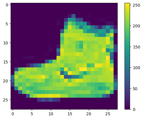
在將這些值饋送到神經網路模型之前，請將其縮放至 0 到 1 的範圍。若要執行此操作，請將值除以 255。訓練集和測試集必須以相同方式預先處理，這一點很重要

train_images = train_images / 255.0

test_images = test_images / 255.0

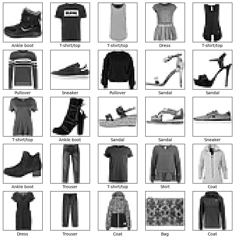
為了驗證資料格式是否正確，以及您是否已準備好建構和訓練網路，讓我們顯示來自訓練集的前 25 張圖片，並在每張圖片下方顯示類別名稱。

plt.figure(figsize=(10,10))
for i in range(25):
    plt.subplot(5,5,i+1)
    plt.xticks([])
    plt.yticks([])
    plt.grid(False)
    plt.imshow(train_images[i], cmap=plt.cm.binary)
    plt.xlabel(class_names[train_labels[i]])
plt.show()

建構模型

建構神經網路需要設定模型的層，然後編譯模型。

設定層

神經網路的基本建構區塊是層。層會從饋送到其中的資料中擷取表示法。理想情況下，這些表示法對於手邊的問題來說是有意義的。

大部分的深度學習都包含將簡單層鏈結在一起。大部分的層 (例如 tf.keras.layers.Dense) 都有在訓練期間學習的參數。

model = tf.keras.Sequential([
    tf.keras.layers.Flatten(input_shape=(28, 28)),
    tf.keras.layers.Dense(128, activation='relu'),
    tf.keras.layers.Dense(10)
])

/tmpfs/src/tf_docs_env/lib/python3.9/site-packages/keras/src/layers/reshaping/flatten.py:37: UserWarning: Do not pass an `input_shape`/`input_dim` argument to a layer. When using Sequential models, prefer using an `Input(shape)` object as the first layer in the model instead.
  super().__init__(**kwargs)

此網路中的第一層 tf.keras.layers.Flatten 會將圖片的格式從二維陣列 (28 x 28 像素) 轉換為一維陣列 (28 * 28 = 784 像素)。您可以將此層視為展開圖片中的像素列並將其排列起來。此層沒有要學習的參數；它只會重新格式化資料。

在像素展平之後，網路會包含兩個 tf.keras.layers.Dense 層的序列。這些是密集連線或完全連線的神經層。第一個 Dense 層有 128 個節點 (或神經元)。第二個 (也是最後一個) 層會傳回長度為 10 的 logits 陣列。每個節點都包含一個分數，指出目前圖片屬於 10 個類別中的哪一個。

編譯模型

在模型準備好進行訓練之前，還需要一些設定。這些設定是在模型的編譯步驟中新增的

• 最佳化工具 — 這是模型根據其看到的資料及其損失函數進行更新的方式。
• 損失函數 — 這會測量模型在訓練期間的準確度。您會想要盡可能縮小此函數，以便將模型「引導」到正確的方向。
• 指標 — 用於監控訓練和測試步驟。以下範例使用準確度，也就是正確分類的圖片比例。

model.compile(optimizer='adam',
              loss=tf.keras.losses.SparseCategoricalCrossentropy(from_logits=True),
              metrics=['accuracy'])

訓練模型

訓練神經網路模型需要執行下列步驟

1. 將訓練資料饋送到模型。在本範例中，訓練資料位於 train_images 和 train_labels 陣列中。
2. 模型學習將圖片和標籤建立關聯。
3. 您要求模型針對測試集 (在本範例中為 test_images 陣列) 做出預測。
4. 驗證預測是否與 test_labels 陣列中的標籤相符。

饋送模型

若要開始訓練，請呼叫 model.fit 方法，之所以如此命名是因為它會將模型「擬合」到訓練資料

model.fit(train_images, train_labels, epochs=10)

Epoch 1/10
WARNING: All log messages before absl::InitializeLog() is called are written to STDERR
I0000 00:00:1720844382.080422   73401 service.cc:145] XLA service 0x7f7a68006fc0 initialized for platform CUDA (this does not guarantee that XLA will be used). Devices:
I0000 00:00:1720844382.080462   73401 service.cc:153]   StreamExecutor device (0): Tesla T4, Compute Capability 7.5
I0000 00:00:1720844382.080467   73401 service.cc:153]   StreamExecutor device (1): Tesla T4, Compute Capability 7.5
I0000 00:00:1720844382.080470   73401 service.cc:153]   StreamExecutor device (2): Tesla T4, Compute Capability 7.5
I0000 00:00:1720844382.080473   73401 service.cc:153]   StreamExecutor device (3): Tesla T4, Compute Capability 7.5
124/1875 ━━━━━━━━━━━━━━━━━━━━ 2s 1ms/step - accuracy: 0.5870 - loss: 1.2303
I0000 00:00:1720844382.812309   73401 device_compiler.h:188] Compiled cluster using XLA!  This line is logged at most once for the lifetime of the process.
1875/1875 ━━━━━━━━━━━━━━━━━━━━ 4s 1ms/step - accuracy: 0.7832 - loss: 0.6298
Epoch 2/10
1875/1875 ━━━━━━━━━━━━━━━━━━━━ 2s 1ms/step - accuracy: 0.8619 - loss: 0.3838
Epoch 3/10
1875/1875 ━━━━━━━━━━━━━━━━━━━━ 2s 1ms/step - accuracy: 0.8715 - loss: 0.3471
Epoch 4/10
1875/1875 ━━━━━━━━━━━━━━━━━━━━ 2s 1ms/step - accuracy: 0.8866 - loss: 0.3164
Epoch 5/10
1875/1875 ━━━━━━━━━━━━━━━━━━━━ 2s 1ms/step - accuracy: 0.8936 - loss: 0.2910
Epoch 6/10
1875/1875 ━━━━━━━━━━━━━━━━━━━━ 2s 1ms/step - accuracy: 0.8978 - loss: 0.2773
Epoch 7/10
1875/1875 ━━━━━━━━━━━━━━━━━━━━ 2s 1ms/step - accuracy: 0.8998 - loss: 0.2653
Epoch 8/10
1875/1875 ━━━━━━━━━━━━━━━━━━━━ 2s 1ms/step - accuracy: 0.9039 - loss: 0.2578
Epoch 9/10
1875/1875 ━━━━━━━━━━━━━━━━━━━━ 2s 1ms/step - accuracy: 0.9079 - loss: 0.2458
Epoch 10/10
1875/1875 ━━━━━━━━━━━━━━━━━━━━ 2s 1ms/step - accuracy: 0.9149 - loss: 0.2300
<keras.src.callbacks.history.History at 0x7f7c3b75e7c0>

在模型訓練時，會顯示損失和準確度指標。此模型在訓練資料上的準確度達到約 0.91 (或 91%)。

評估準確度

接下來，比較模型在測試資料集上的效能

test_loss, test_acc = model.evaluate(test_images,  test_labels, verbose=2)

print('\nTest accuracy:', test_acc)

313/313 - 1s - 3ms/step - accuracy: 0.8888 - loss: 0.3224

Test accuracy: 0.8888000249862671

結果顯示，測試資料集的準確度略低於訓練資料集的準確度。訓練準確度和測試準確度之間的這種差距代表過度擬合。當機器學習模型在新、先前未見過的輸入上的效能比在訓練資料上的效能更差時，就會發生過度擬合。過度擬合的模型會「記住」訓練資料集中的雜訊和細節，以至於對模型在新資料上的效能產生負面影響。如需更多資訊，請參閱下列內容

• 示範過度擬合
• 防止過度擬合的策略

做出預測

在模型訓練完成後，您可以使用它來預測某些圖片。附加 softmax 層以轉換模型的線性輸出 (logits) 為機率，這樣應該更容易解讀。

probability_model = tf.keras.Sequential([model, 
                                         tf.keras.layers.Softmax()])

predictions = probability_model.predict(test_images)

313/313 ━━━━━━━━━━━━━━━━━━━━ 1s 1ms/step

在這裡，模型已預測測試集中每張圖片的標籤。讓我們看看第一個預測

predictions[0]

array([1.0297459e-08, 6.0991318e-10, 4.4771734e-10, 4.6667561e-12,
       1.7007395e-08, 2.9962388e-04, 1.6731771e-07, 2.5453644e-03,
       3.6041616e-08, 9.9715471e-01], dtype=float32)

預測是 10 個數字的陣列。它們代表模型「確信」圖片對應到 10 種不同服裝單品中每一種的程度。您可以查看哪個標籤具有最高的信賴度值

np.argmax(predictions[0])

9

因此，模型最確信此圖片是踝靴，或 class_names[9]。檢查測試標籤會顯示此分類是正確的

test_labels[0]

9

定義函數以繪製完整 10 個類別預測的圖表。

def plot_image(i, predictions_array, true_label, img):
  true_label, img = true_label[i], img[i]
  plt.grid(False)
  plt.xticks([])
  plt.yticks([])

  plt.imshow(img, cmap=plt.cm.binary)

  predicted_label = np.argmax(predictions_array)
  if predicted_label == true_label:
    color = 'blue'
  else:
    color = 'red'

  plt.xlabel("{} {:2.0f}% ({})".format(class_names[predicted_label],
                                100*np.max(predictions_array),
                                class_names[true_label]),
                                color=color)

def plot_value_array(i, predictions_array, true_label):
  true_label = true_label[i]
  plt.grid(False)
  plt.xticks(range(10))
  plt.yticks([])
  thisplot = plt.bar(range(10), predictions_array, color="#777777")
  plt.ylim([0, 1])
  predicted_label = np.argmax(predictions_array)

  thisplot[predicted_label].set_color('red')
  thisplot[true_label].set_color('blue')

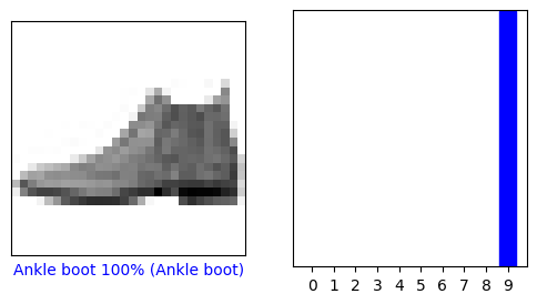
驗證預測

在模型訓練完成後，您可以使用它來預測某些圖片。

讓我們看看第 0 張圖片、預測和預測陣列。正確預測標籤為藍色，不正確預測標籤為紅色。數字表示預測標籤的百分比 (滿分 100%)。

i = 0
plt.figure(figsize=(6,3))
plt.subplot(1,2,1)
plot_image(i, predictions[i], test_labels, test_images)
plt.subplot(1,2,2)
plot_value_array(i, predictions[i],  test_labels)
plt.show()

i = 12
plt.figure(figsize=(6,3))
plt.subplot(1,2,1)
plot_image(i, predictions[i], test_labels, test_images)
plt.subplot(1,2,2)
plot_value_array(i, predictions[i],  test_labels)
plt.show()

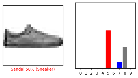
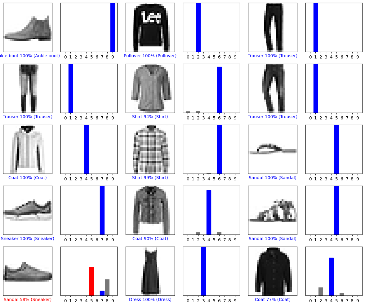
讓我們繪製幾張圖片及其預測結果。請注意，即使模型非常有信心，也可能會出錯。

# Plot the first X test images, their predicted labels, and the true labels.
# Color correct predictions in blue and incorrect predictions in red.
num_rows = 5
num_cols = 3
num_images = num_rows*num_cols
plt.figure(figsize=(2*2*num_cols, 2*num_rows))
for i in range(num_images):
  plt.subplot(num_rows, 2*num_cols, 2*i+1)
  plot_image(i, predictions[i], test_labels, test_images)
  plt.subplot(num_rows, 2*num_cols, 2*i+2)
  plot_value_array(i, predictions[i], test_labels)
plt.tight_layout()
plt.show()

使用已訓練的模型

最後，使用已訓練的模型來預測單張圖片。

# Grab an image from the test dataset.
img = test_images[1]

print(img.shape)

(28, 28)

tf.keras 模型經過最佳化，可一次對一批或一組範例進行預測。因此，即使您使用的是單張圖片，您也需要將它新增至清單

# Add the image to a batch where it's the only member.
img = (np.expand_dims(img,0))

print(img.shape)

(1, 28, 28)

現在預測此圖片的正確標籤

predictions_single = probability_model.predict(img)

print(predictions_single)

1/1 ━━━━━━━━━━━━━━━━━━━━ 0s 140ms/step
[[3.1302361e-06 2.6202183e-12 9.9640650e-01 3.0387102e-13 3.1137168e-03
  5.0210312e-11 4.7672543e-04 8.7875020e-13 4.1576378e-11 2.9291714e-15]]

plot_value_array(1, predictions_single[0], test_labels)
_ = plt.xticks(range(10), class_names, rotation=45)
plt.show()

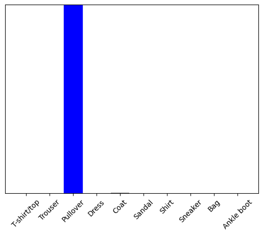
tf.keras.Model.predict 會傳回清單的清單，批次資料中的每張圖片都有一個清單。擷取批次中 (唯一) 圖片的預測

np.argmax(predictions_single[0])

2

而且模型會如預期般預測標籤。

若要進一步瞭解如何使用 Keras 建構模型，請參閱 Keras 指南。

# MIT License
#
# Copyright (c) 2017 François Chollet
#
# Permission is hereby granted, free of charge, to any person obtaining a
# copy of this software and associated documentation files (the "Software"),
# to deal in the Software without restriction, including without limitation
# the rights to use, copy, modify, merge, publish, distribute, sublicense,
# and/or sell copies of the Software, and to permit persons to whom the
# Software is furnished to do so, subject to the following conditions:
#
# The above copyright notice and this permission notice shall be included in
# all copies or substantial portions of the Software.
#
# THE SOFTWARE IS PROVIDED "AS IS", WITHOUT WARRANTY OF ANY KIND, EXPRESS OR
# IMPLIED, INCLUDING BUT NOT LIMITED TO THE WARRANTIES OF MERCHANTABILITY,
# FITNESS FOR A PARTICULAR PURPOSE AND NONINFRINGEMENT. IN NO EVENT SHALL
# THE AUTHORS OR COPYRIGHT HOLDERS BE LIABLE FOR ANY CLAIM, DAMAGES OR OTHER
# LIABILITY, WHETHER IN AN ACTION OF CONTRACT, TORT OR OTHERWISE, ARISING
# FROM, OUT OF OR IN CONNECTION WITH THE SOFTWARE OR THE USE OR OTHER
# DEALINGS IN THE SOFTWARE.