
|
|
|
 在 GitHub 上檢視原始碼 在 GitHub 上檢視原始碼
|
|
本教學課程示範如何訓練簡易的卷積神經網路 (CNN) 來分類 CIFAR 圖片。由於本教學課程使用 Keras Sequential API,因此建立和訓練模型只需幾行程式碼。
匯入 TensorFlow
import tensorflow as tf

from tensorflow.keras import datasets, layers, models
import matplotlib.pyplot as plt
2023-10-27 06:01:15.153603: E external/local_xla/xla/stream_executor/cuda/cuda_dnn.cc:9261] Unable to register cuDNN factory: Attempting to register factory for plugin cuDNN when one has already been registered
2023-10-27 06:01:15.153656: E external/local_xla/xla/stream_executor/cuda/cuda_fft.cc:607] Unable to register cuFFT factory: Attempting to register factory for plugin cuFFT when one has already been registered
2023-10-27 06:01:15.155401: E external/local_xla/xla/stream_executor/cuda/cuda_blas.cc:1515] Unable to register cuBLAS factory: Attempting to register factory for plugin cuBLAS when one has already been registered
下載並準備 CIFAR10 資料集
CIFAR10 資料集包含 60,000 張彩色圖片,分為 10 個類別,每個類別有 6,000 張圖片。資料集分為 50,000 張訓練圖片和 10,000 張測試圖片。類別之間互斥,且彼此之間沒有重疊。
(train_images, train_labels), (test_images, test_labels) = datasets.cifar10.load_data()

# Normalize pixel values to be between 0 and 1
train_images, test_images = train_images / 255.0, test_images / 255.0
Downloading data from https://www.cs.toronto.edu/~kriz/cifar-10-python.tar.gz
170498071/170498071 [==============================] - 2s 0us/step
驗證資料
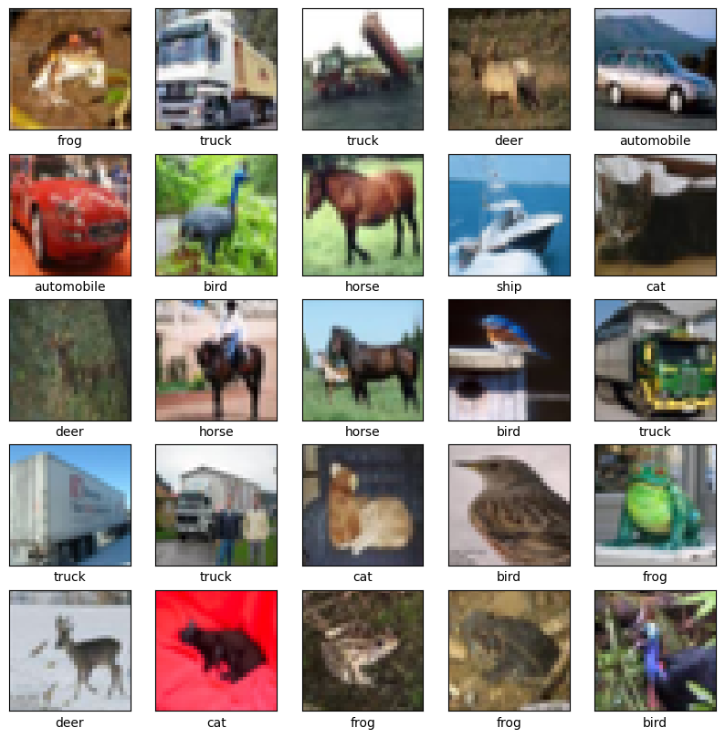
為了驗證資料集看起來是否正確,我們繪製訓練集中的前 25 張圖片,並在每張圖片下方顯示類別名稱
class_names = ['airplane', 'automobile', 'bird', 'cat', 'deer',
               'dog', 'frog', 'horse', 'ship', 'truck']

plt.figure(figsize=(10,10))
for i in range(25):
    plt.subplot(5,5,i+1)
    plt.xticks([])
    plt.yticks([])
    plt.grid(False)
    plt.imshow(train_images[i])
    # The CIFAR labels happen to be arrays,
    # which is why you need the extra index
    plt.xlabel(class_names[train_labels[i][0]])
plt.show()
建立卷積基底
以下 6 行程式碼使用常見模式定義卷積基底:Conv2D 和 MaxPooling2D 層的堆疊。
作為輸入,CNN 接受形狀為 (image_height, image_width, color_channels) 的張量,並忽略批次大小。如果您不熟悉這些維度,color_channels 是指 (R,G,B)。在本範例中,您將設定 CNN 處理形狀為 (32, 32, 3) 的輸入,這是 CIFAR 圖片的格式。您可以透過將引數 input_shape 傳遞至第一層來完成此操作。
model = models.Sequential()
model.add(layers.Conv2D(32, (3, 3), activation='relu', input_shape=(32, 32, 3)))
model.add(layers.MaxPooling2D((2, 2)))
model.add(layers.Conv2D(64, (3, 3), activation='relu'))
model.add(layers.MaxPooling2D((2, 2)))
model.add(layers.Conv2D(64, (3, 3), activation='relu'))
讓我們顯示目前模型的架構
model.summary()
Model: "sequential"
_________________________________________________________________
 Layer (type)                Output Shape              Param #
=================================================================
 conv2d (Conv2D)             (None, 30, 30, 32)        896

 max_pooling2d (MaxPooling2  (None, 15, 15, 32)        0
 D)

 conv2d_1 (Conv2D)           (None, 13, 13, 64)        18496

 max_pooling2d_1 (MaxPoolin  (None, 6, 6, 64)          0
 g2D)

 conv2d_2 (Conv2D)           (None, 4, 4, 64)          36928

=================================================================
Total params: 56320 (220.00 KB)
Trainable params: 56320 (220.00 KB)
Non-trainable params: 0 (0.00 Byte)
_________________________________________________________________
在上方,您可以看到每個 Conv2D 和 MaxPooling2D 層的輸出都是形狀為 (height, width, channels) 的 3D 張量。當您在網路中深入時,寬度和高度維度會趨於縮小。每個 Conv2D 層的輸出通道數由第一個引數 (例如 32 或 64) 控制。通常,隨著寬度和高度縮小,您可以在每個 Conv2D 層中新增更多輸出通道 (以運算方式來說)。
在頂端新增密集層
為了完成模型,您會將卷積基底的最後一個輸出張量 (形狀為 (4, 4, 64)) 饋送至一或多個密集層以執行分類。密集層以向量 (1D) 作為輸入,而目前的輸出是 3D 張量。首先,您會將 3D 輸出扁平化 (或展開) 為 1D,然後在頂端新增一或多個密集層。CIFAR 有 10 個輸出類別,因此您使用具有 10 個輸出的最終密集層。
model.add(layers.Flatten())
model.add(layers.Dense(64, activation='relu'))
model.add(layers.Dense(10))
以下是您模型的完整架構
model.summary()
Model: "sequential"
_________________________________________________________________
 Layer (type)                Output Shape              Param #
=================================================================
 conv2d (Conv2D)             (None, 30, 30, 32)        896

 max_pooling2d (MaxPooling2  (None, 15, 15, 32)        0
 D)

 conv2d_1 (Conv2D)           (None, 13, 13, 64)        18496

 max_pooling2d_1 (MaxPoolin  (None, 6, 6, 64)          0
 g2D)

 conv2d_2 (Conv2D)           (None, 4, 4, 64)          36928

 flatten (Flatten)           (None, 1024)              0

 dense (Dense)               (None, 64)                65600

 dense_1 (Dense)             (None, 10)                650

=================================================================
Total params: 122570 (478.79 KB)
Trainable params: 122570 (478.79 KB)
Non-trainable params: 0 (0.00 Byte)
_________________________________________________________________
網路摘要顯示 (4, 4, 64) 輸出在經過兩個密集層之前已扁平化為形狀為 (1024) 的向量。
編譯並訓練模型
model.compile(optimizer='adam',
              loss=tf.keras.losses.SparseCategoricalCrossentropy(from_logits=True),
              metrics=['accuracy'])

history = model.fit(train_images, train_labels, epochs=10,
                    validation_data=(test_images, test_labels))
Epoch 1/10
WARNING: All log messages before absl::InitializeLog() is called are written to STDERR
I0000 00:00:1698386490.372362  489369 device_compiler.h:186] Compiled cluster using XLA!  This line is logged at most once for the lifetime of the process.
1563/1563 [==============================] - 10s 5ms/step - loss: 1.5211 - accuracy: 0.4429 - val_loss: 1.2497 - val_accuracy: 0.5531
Epoch 2/10
1563/1563 [==============================] - 6s 4ms/step - loss: 1.1408 - accuracy: 0.5974 - val_loss: 1.1474 - val_accuracy: 0.6023
Epoch 3/10
1563/1563 [==============================] - 6s 4ms/step - loss: 0.9862 - accuracy: 0.6538 - val_loss: 0.9759 - val_accuracy: 0.6582
Epoch 4/10
1563/1563 [==============================] - 6s 4ms/step - loss: 0.8929 - accuracy: 0.6879 - val_loss: 0.9412 - val_accuracy: 0.6702
Epoch 5/10
1563/1563 [==============================] - 6s 4ms/step - loss: 0.8183 - accuracy: 0.7131 - val_loss: 0.8830 - val_accuracy: 0.6967
Epoch 6/10
1563/1563 [==============================] - 6s 4ms/step - loss: 0.7588 - accuracy: 0.7334 - val_loss: 0.8671 - val_accuracy: 0.7039
Epoch 7/10
1563/1563 [==============================] - 6s 4ms/step - loss: 0.7126 - accuracy: 0.7518 - val_loss: 0.8972 - val_accuracy: 0.6897
Epoch 8/10
1563/1563 [==============================] - 7s 4ms/step - loss: 0.6655 - accuracy: 0.7661 - val_loss: 0.8412 - val_accuracy: 0.7111
Epoch 9/10
1563/1563 [==============================] - 7s 4ms/step - loss: 0.6205 - accuracy: 0.7851 - val_loss: 0.8581 - val_accuracy: 0.7109
Epoch 10/10
1563/1563 [==============================] - 7s 4ms/step - loss: 0.5872 - accuracy: 0.7937 - val_loss: 0.8817 - val_accuracy: 0.7113
評估模型
plt.plot(history.history['accuracy'], label='accuracy')
plt.plot(history.history['val_accuracy'], label = 'val_accuracy')
plt.xlabel('Epoch')
plt.ylabel('Accuracy')
plt.ylim([0.5, 1])
plt.legend(loc='lower right')

test_loss, test_acc = model.evaluate(test_images,  test_labels, verbose=2)
313/313 - 1s - loss: 0.8817 - accuracy: 0.7113 - 655ms/epoch - 2ms/step
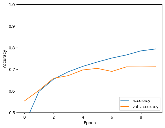
print(test_acc)
0.7113000154495239
您的簡易 CNN 已達到超過 70% 的測試準確度。以幾行程式碼來說,還算不錯!如需其他 CNN 樣式,請查看 TensorFlow 2 專家快速入門範例,其中使用 Keras 子類別化 API 和 tf.GradientTape。