
|
|
|
 在 GitHub 上檢視 在 GitHub 上檢視
|
|
|
本教學課程使用深度學習將一張影像以另一張影像的風格合成(是否曾希望自己能像畢卡索或梵谷一樣作畫?)。這稱為「神經風格轉換」,此技術概述於藝術風格的神經演算法 (Gatys et al.)。
如需搭配 TensorFlow Hub 預訓練模型進行風格轉換的簡單應用,請查看適用於任意風格的快速風格轉換教學課程,其中使用任意影像風格化模型。如需搭配 TensorFlow Lite 進行風格轉換的範例,請參閱使用 TensorFlow Lite 進行藝術風格轉換。
神經風格轉換是一種最佳化技術,用於取得兩張影像,即一張「內容」影像和一張「風格參考」影像(例如著名畫家的藝術作品),並將它們混合在一起,使輸出影像看起來像內容影像,但以風格參考影像的風格「繪製」。
這是透過最佳化輸出影像,使其符合內容影像的內容統計資料和風格參考影像的風格統計資料來實作。這些統計資料是使用卷積網路從影像中擷取出來的。
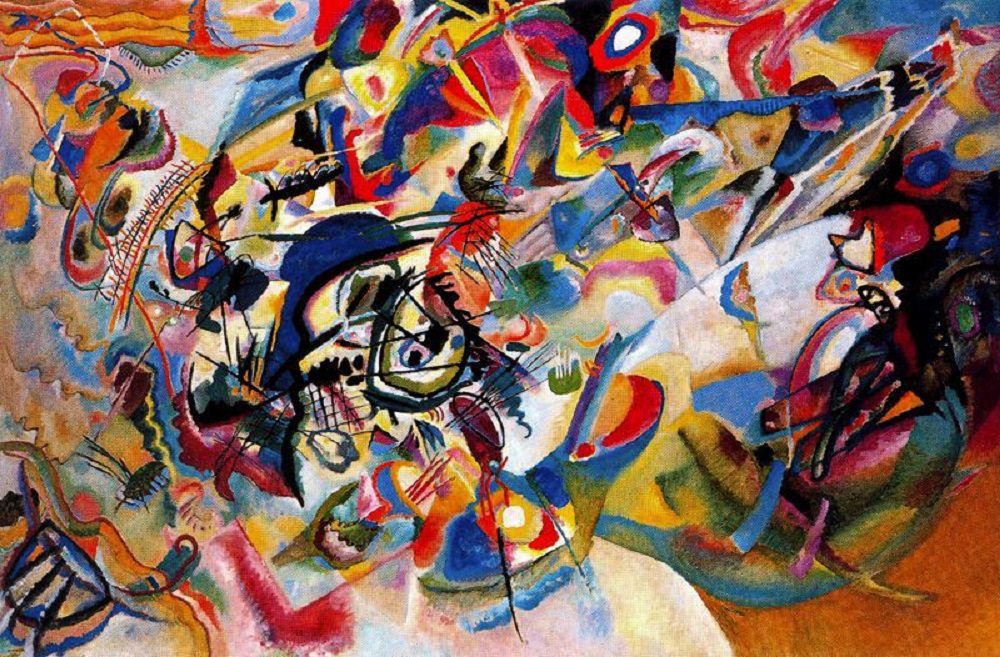
例如,讓我們以這隻狗的影像和 Wassily Kandinsky 的《Composition 7》為例
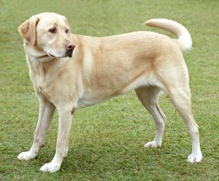
黃色拉布拉多犬觀看,來自 Wikimedia Commons,作者:Elf。授權條款 CC BY-SA 3.0
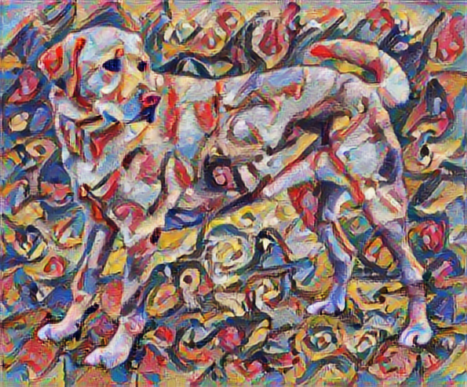
那麼,如果康丁斯基決定完全以這種風格繪製這隻狗的圖片,會是什麼樣子呢?像這樣嗎?

設定
匯入並設定模組
import os
import tensorflow as tf
# Load compressed models from tensorflow_hub
os.environ['TFHUB_MODEL_LOAD_FORMAT'] = 'COMPRESSED'
import IPython.display as display

import matplotlib.pyplot as plt
import matplotlib as mpl
mpl.rcParams['figure.figsize'] = (12, 12)
mpl.rcParams['axes.grid'] = False

import numpy as np
import PIL.Image
import time
import functools
def tensor_to_image(tensor):
  tensor = tensor*255
  tensor = np.array(tensor, dtype=np.uint8)
  if np.ndim(tensor)>3:
    assert tensor.shape[0] == 1
    tensor = tensor[0]
  return PIL.Image.fromarray(tensor)
下載影像並選擇風格影像和內容影像
content_path = tf.keras.utils.get_file('YellowLabradorLooking_new.jpg', 'https://storage.googleapis.com/download.tensorflow.org/example_images/YellowLabradorLooking_new.jpg')
style_path = tf.keras.utils.get_file('kandinsky5.jpg','https://storage.googleapis.com/download.tensorflow.org/example_images/Vassily_Kandinsky%2C_1913_-_Composition_7.jpg')
Downloading data from https://storage.googleapis.com/download.tensorflow.org/example_images/YellowLabradorLooking_new.jpg
83281/83281 ━━━━━━━━━━━━━━━━━━━━ 0s 0us/step
Downloading data from https://storage.googleapis.com/download.tensorflow.org/example_images/Vassily_Kandinsky%2C_1913_-_Composition_7.jpg
195196/195196 ━━━━━━━━━━━━━━━━━━━━ 0s 0us/step
可視化輸入
定義一個函數來載入影像,並將其最大尺寸限制為 512 像素。
def load_img(path_to_img):
  max_dim = 512
  img = tf.io.read_file(path_to_img)
  img = tf.image.decode_image(img, channels=3)
  img = tf.image.convert_image_dtype(img, tf.float32)

  shape = tf.cast(tf.shape(img)[:-1], tf.float32)
  long_dim = max(shape)
  scale = max_dim / long_dim

  new_shape = tf.cast(shape * scale, tf.int32)

  img = tf.image.resize(img, new_shape)
  img = img[tf.newaxis, :]
  return img
建立一個簡單的函數來顯示影像
def imshow(image, title=None):
  if len(image.shape) > 3:
    image = tf.squeeze(image, axis=0)

  plt.imshow(image)
  if title:
    plt.title(title)
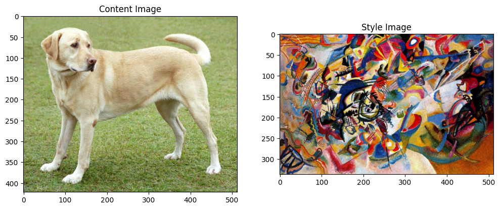
content_image = load_img(content_path)
style_image = load_img(style_path)

plt.subplot(1, 2, 1)
imshow(content_image, 'Content Image')

plt.subplot(1, 2, 2)
imshow(style_image, 'Style Image')
使用 TF-Hub 進行快速風格轉換
本教學課程示範原始的風格轉換演算法,它將影像內容最佳化為特定風格。在深入探討細節之前,讓我們先看看 TensorFlow Hub 模型是如何做到這一點的
import tensorflow_hub as hub
hub_model = hub.load('https://tfhub.dev/google/magenta/arbitrary-image-stylization-v1-256/2')
stylized_image = hub_model(tf.constant(content_image), tf.constant(style_image))[0]
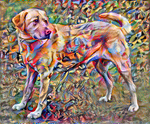
tensor_to_image(stylized_image)
定義內容和風格表示法
使用模型的中間層來取得影像的內容和風格表示法。從網路的輸入層開始,前幾個層的啟動代表低階特徵,例如邊緣和紋理。當您逐步瀏覽網路時,最後幾個層代表高階特徵,即物件部分,例如輪子或眼睛。在本例中,您使用的是 VGG19 網路架構,這是一個預訓練的影像分類網路。這些中間層對於定義影像的內容和風格表示法是必要的。對於輸入影像,請嘗試在這些中間層中比對對應的風格和內容目標表示法。
載入 VGG19 並在我們的影像上測試執行,以確保其使用正確
x = tf.keras.applications.vgg19.preprocess_input(content_image*255)
x = tf.image.resize(x, (224, 224))
vgg = tf.keras.applications.VGG19(include_top=True, weights='imagenet')
prediction_probabilities = vgg(x)
prediction_probabilities.shape
Downloading data from https://storage.googleapis.com/tensorflow/keras-applications/vgg19/vgg19_weights_tf_dim_ordering_tf_kernels.h5
574710816/574710816 ━━━━━━━━━━━━━━━━━━━━ 10s 0us/step
TensorShape([1, 1000])
predicted_top_5 = tf.keras.applications.vgg19.decode_predictions(prediction_probabilities.numpy())[0]
[(class_name, prob) for (number, class_name, prob) in predicted_top_5]
Downloading data from https://storage.googleapis.com/download.tensorflow.org/data/imagenet_class_index.json
35363/35363 ━━━━━━━━━━━━━━━━━━━━ 0s 0us/step
[('Labrador_retriever', 0.49317107),
 ('golden_retriever', 0.23665293),
 ('kuvasz', 0.03635751),
 ('Chesapeake_Bay_retriever', 0.024182767),
 ('Greater_Swiss_Mountain_dog', 0.018646102)]
現在載入沒有分類標頭的 VGG19,並列出層名稱
vgg = tf.keras.applications.VGG19(include_top=False, weights='imagenet')

print()
for layer in vgg.layers:
  print(layer.name)
Downloading data from https://storage.googleapis.com/tensorflow/keras-applications/vgg19/vgg19_weights_tf_dim_ordering_tf_kernels_notop.h5
80134624/80134624 ━━━━━━━━━━━━━━━━━━━━ 0s 0us/step

input_layer_1
block1_conv1
block1_conv2
block1_pool
block2_conv1
block2_conv2
block2_pool
block3_conv1
block3_conv2
block3_conv3
block3_conv4
block3_pool
block4_conv1
block4_conv2
block4_conv3
block4_conv4
block4_pool
block5_conv1
block5_conv2
block5_conv3
block5_conv4
block5_pool
從網路中選擇中間層來表示影像的風格和內容
content_layers = ['block5_conv2']

style_layers = ['block1_conv1',
                'block2_conv1',
                'block3_conv1',
                'block4_conv1',
                'block5_conv1']

num_content_layers = len(content_layers)
num_style_layers = len(style_layers)
風格和內容的中間層
那麼,為什麼我們預訓練的影像分類網路中的這些中間輸出,能夠讓我們定義風格和內容表示法呢?
從高層次來看,為了讓網路執行影像分類(這個網路已經過訓練來執行此操作),它必須理解影像。這需要將原始影像作為輸入像素,並建立一個內部表示法,將原始影像像素轉換為對影像內存在的特徵的複雜理解。
這也是卷積神經網路能夠很好地泛化的原因:它們能夠捕捉類別內的恆定性和定義特徵(例如貓與狗),這些特徵與背景雜訊和其他干擾無關。因此,在原始影像饋送到模型和輸出分類標籤之間,模型充當複雜的特徵擷取器。透過存取模型的中間層,您可以描述輸入影像的內容和風格。
建構模型
tf.keras.applications 中的網路經過設計,因此您可以使用 Keras functional API 輕鬆擷取中間層值。
若要使用 functional API 定義模型,請指定輸入和輸出
model = Model(inputs, outputs)
以下函數會建構一個 VGG19 模型,該模型會傳回中間層輸出的清單
def vgg_layers(layer_names):
  """ Creates a VGG model that returns a list of intermediate output values."""
  # Load our model. Load pretrained VGG, trained on ImageNet data
  vgg = tf.keras.applications.VGG19(include_top=False, weights='imagenet')
  vgg.trainable = False

  outputs = [vgg.get_layer(name).output for name in layer_names]

  model = tf.keras.Model([vgg.input], outputs)
  return model
以及建立模型
style_extractor = vgg_layers(style_layers)
style_outputs = style_extractor(style_image*255)

#Look at the statistics of each layer's output
for name, output in zip(style_layers, style_outputs):
  print(name)
  print("  shape: ", output.numpy().shape)
  print("  min: ", output.numpy().min())
  print("  max: ", output.numpy().max())
  print("  mean: ", output.numpy().mean())
  print()
block1_conv1
  shape:  (1, 336, 512, 64)
  min:  0.0
  max:  835.5256
  mean:  33.97525

block2_conv1
  shape:  (1, 168, 256, 128)
  min:  0.0
  max:  4625.8857
  mean:  199.82687

block3_conv1
  shape:  (1, 84, 128, 256)
  min:  0.0
  max:  8789.239
  mean:  230.78099

block4_conv1
  shape:  (1, 42, 64, 512)
  min:  0.0
  max:  21566.135
  mean:  791.24005

block5_conv1
  shape:  (1, 21, 32, 512)
  min:  0.0
  max:  3189.2542
  mean:  59.179478
計算風格
影像的內容由中間特徵圖的值表示。
事實證明,影像的風格可以用不同特徵圖之間的均值和相關性來描述。計算包含此資訊的 Gram 矩陣,方法是在每個位置取得特徵向量與其自身的外部乘積,並對所有位置的外部乘積求平均值。此 Gram 矩陣可以針對特定層計算為
\[G^l_{cd} = \frac{\sum_{ij} F^l_{ijc}(x)F^l_{ijd}(x)}{IJ}\]
這可以使用 tf.linalg.einsum 函數簡潔地實作
def gram_matrix(input_tensor):
  result = tf.linalg.einsum('bijc,bijd->bcd', input_tensor, input_tensor)
  input_shape = tf.shape(input_tensor)
  num_locations = tf.cast(input_shape[1]*input_shape[2], tf.float32)
  return result/(num_locations)
擷取風格和內容
建構一個傳回風格和內容張量的模型。
class StyleContentModel(tf.keras.models.Model):
  def __init__(self, style_layers, content_layers):
    super(StyleContentModel, self).__init__()
    self.vgg = vgg_layers(style_layers + content_layers)
    self.style_layers = style_layers
    self.content_layers = content_layers
    self.num_style_layers = len(style_layers)
    self.vgg.trainable = False

  def call(self, inputs):
    "Expects float input in [0,1]"
    inputs = inputs*255.0
    preprocessed_input = tf.keras.applications.vgg19.preprocess_input(inputs)
    outputs = self.vgg(preprocessed_input)
    style_outputs, content_outputs = (outputs[:self.num_style_layers],
                                      outputs[self.num_style_layers:])

    style_outputs = [gram_matrix(style_output)
                     for style_output in style_outputs]

    content_dict = {content_name: value
                    for content_name, value
                    in zip(self.content_layers, content_outputs)}

    style_dict = {style_name: value
                  for style_name, value
                  in zip(self.style_layers, style_outputs)}

    return {'content': content_dict, 'style': style_dict}
當在影像上呼叫時,此模型會傳回 style_layers 的 gram 矩陣(風格)和 content_layers 的內容
extractor = StyleContentModel(style_layers, content_layers)

results = extractor(tf.constant(content_image))

print('Styles:')
for name, output in sorted(results['style'].items()):
  print("  ", name)
  print("    shape: ", output.numpy().shape)
  print("    min: ", output.numpy().min())
  print("    max: ", output.numpy().max())
  print("    mean: ", output.numpy().mean())
  print()

print("Contents:")
for name, output in sorted(results['content'].items()):
  print("  ", name)
  print("    shape: ", output.numpy().shape)
  print("    min: ", output.numpy().min())
  print("    max: ", output.numpy().max())
  print("    mean: ", output.numpy().mean())
Styles:
   block1_conv1
    shape:  (1, 64, 64)
    min:  0.005522845
    max:  28014.555
    mean:  263.79022

   block2_conv1
    shape:  (1, 128, 128)
    min:  0.0
    max:  61479.484
    mean:  9100.949

   block3_conv1
    shape:  (1, 256, 256)
    min:  0.0
    max:  545623.44
    mean:  7660.976

   block4_conv1
    shape:  (1, 512, 512)
    min:  0.0
    max:  4320502.0
    mean:  134288.84

   block5_conv1
    shape:  (1, 512, 512)
    min:  0.0
    max:  110005.37
    mean:  1487.0378

Contents:
   block5_conv2
    shape:  (1, 26, 32, 512)
    min:  0.0
    max:  2410.8796
    mean:  13.764149
執行梯度下降
有了這個風格和內容擷取器,您現在可以實作風格轉換演算法。方法是計算影像輸出相對於每個目標的均方誤差,然後取這些損失的加權總和。
設定您的風格和內容目標值
style_targets = extractor(style_image)['style']
content_targets = extractor(content_image)['content']
定義一個 tf.Variable 以包含要最佳化的影像。為了加快速度,請使用內容影像初始化它(tf.Variable 必須與內容影像具有相同的形狀)
image = tf.Variable(content_image)
由於這是浮點影像,因此定義一個函數以將像素值保持在 0 到 1 之間
def clip_0_1(image):
  return tf.clip_by_value(image, clip_value_min=0.0, clip_value_max=1.0)
建立最佳化工具。該論文建議使用 LBFGS,但 Adam 也適用
opt = tf.keras.optimizers.Adam(learning_rate=0.02, beta_1=0.99, epsilon=1e-1)
為了最佳化此操作,請使用兩個損失的加權組合來取得總損失
style_weight=1e-2
content_weight=1e4
def style_content_loss(outputs):
    style_outputs = outputs['style']
    content_outputs = outputs['content']
    style_loss = tf.add_n([tf.reduce_mean((style_outputs[name]-style_targets[name])**2)
                           for name in style_outputs.keys()])
    style_loss *= style_weight / num_style_layers

    content_loss = tf.add_n([tf.reduce_mean((content_outputs[name]-content_targets[name])**2)
                             for name in content_outputs.keys()])
    content_loss *= content_weight / num_content_layers
    loss = style_loss + content_loss
    return loss
使用 tf.GradientTape 來更新影像。
@tf.function()
def train_step(image):
  with tf.GradientTape() as tape:
    outputs = extractor(image)
    loss = style_content_loss(outputs)

  grad = tape.gradient(loss, image)
  opt.apply_gradients([(grad, image)])
  image.assign(clip_0_1(image))
現在執行幾個步驟進行測試
train_step(image)
train_step(image)
train_step(image)
tensor_to_image(image)

由於它正在運作,請執行更長時間的最佳化
import time
start = time.time()

epochs = 10
steps_per_epoch = 100

step = 0
for n in range(epochs):
  for m in range(steps_per_epoch):
    step += 1
    train_step(image)
    print(".", end='', flush=True)
  display.clear_output(wait=True)
  display.display(tensor_to_image(image))
  print("Train step: {}".format(step))

end = time.time()
print("Total time: {:.1f}".format(end-start))
Train step: 1000
Total time: 79.0
總變異損失
這個基本實作的一個缺點是它會產生許多高頻率假影。使用影像高頻率成分上的明確正規化項來減少這些假影。在風格轉換中,這通常稱為總變異損失
def high_pass_x_y(image):
  x_var = image[:, :, 1:, :] - image[:, :, :-1, :]
  y_var = image[:, 1:, :, :] - image[:, :-1, :, :]

  return x_var, y_var
x_deltas, y_deltas = high_pass_x_y(content_image)

plt.figure(figsize=(14, 10))
plt.subplot(2, 2, 1)
imshow(clip_0_1(2*y_deltas+0.5), "Horizontal Deltas: Original")

plt.subplot(2, 2, 2)
imshow(clip_0_1(2*x_deltas+0.5), "Vertical Deltas: Original")

x_deltas, y_deltas = high_pass_x_y(image)

plt.subplot(2, 2, 3)
imshow(clip_0_1(2*y_deltas+0.5), "Horizontal Deltas: Styled")

plt.subplot(2, 2, 4)
imshow(clip_0_1(2*x_deltas+0.5), "Vertical Deltas: Styled")
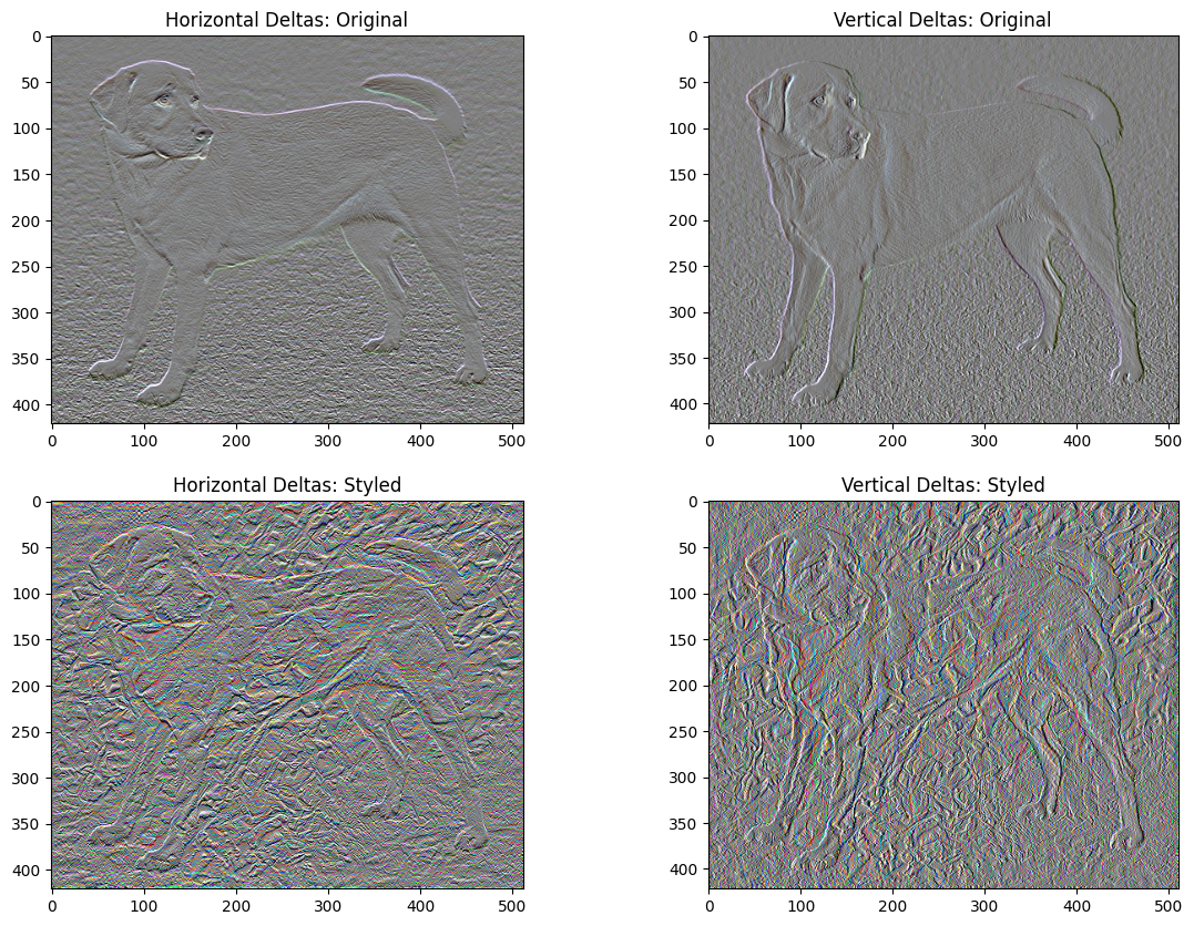
這顯示了高頻率成分是如何增加的。
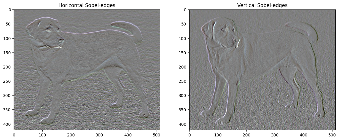
此外,這個高頻率成分基本上是一個邊緣偵測器。例如,您可以從 Sobel 邊緣偵測器獲得類似的輸出。
plt.figure(figsize=(14, 10))

sobel = tf.image.sobel_edges(content_image)
plt.subplot(1, 2, 1)
imshow(clip_0_1(sobel[..., 0]/4+0.5), "Horizontal Sobel-edges")
plt.subplot(1, 2, 2)
imshow(clip_0_1(sobel[..., 1]/4+0.5), "Vertical Sobel-edges")
與此相關的正規化損失是值的平方和
def total_variation_loss(image):
  x_deltas, y_deltas = high_pass_x_y(image)
  return tf.reduce_sum(tf.abs(x_deltas)) + tf.reduce_sum(tf.abs(y_deltas))
total_variation_loss(image).numpy()
149171.38
這示範了它的作用。但沒有必要自己實作,TensorFlow 包含標準實作
tf.image.total_variation(image).numpy()
array([149171.38], dtype=float32)
重新執行最佳化
為 total_variation_loss 選擇權重
total_variation_weight=30
現在將其包含在 train_step 函數中
@tf.function()
def train_step(image):
  with tf.GradientTape() as tape:
    outputs = extractor(image)
    loss = style_content_loss(outputs)
    loss += total_variation_weight*tf.image.total_variation(image)

  grad = tape.gradient(loss, image)
  opt.apply_gradients([(grad, image)])
  image.assign(clip_0_1(image))
重新初始化影像變數和最佳化工具
opt = tf.keras.optimizers.Adam(learning_rate=0.02, beta_1=0.99, epsilon=1e-1)
image = tf.Variable(content_image)
並執行最佳化
import time
start = time.time()

epochs = 10
steps_per_epoch = 100

step = 0
for n in range(epochs):
  for m in range(steps_per_epoch):
    step += 1
    train_step(image)
    print(".", end='', flush=True)
  display.clear_output(wait=True)
  display.display(tensor_to_image(image))
  print("Train step: {}".format(step))

end = time.time()
print("Total time: {:.1f}".format(end-start))
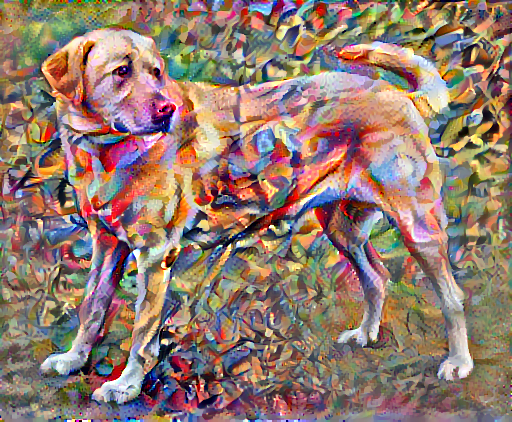
Train step: 1000
Total time: 83.0
最後,儲存結果
file_name = 'stylized-image.png'
tensor_to_image(image).save(file_name)

try:
  from google.colab import files
  files.download(file_name)
except (ImportError, AttributeError):
  pass
深入瞭解
本教學課程示範原始的風格轉換演算法。如需風格轉換的簡單應用,請查看本教學課程,以深入瞭解如何使用 TensorFlow Hub 中的任意影像風格轉換模型。