
|
|
|
 在 GitHub 上查看原始碼 在 GitHub 上查看原始碼
|
|
這個筆記本示範如何在 MNIST 資料集上訓練變分自動編碼器 (VAE) (1、2)。VAE 是自動編碼器的機率版本,自動編碼器是一種模型,可接收高維度輸入資料並將其壓縮成較小的表示法。傳統自動編碼器會將輸入對應到潛在向量,VAE 則不然,它會將輸入資料對應到機率分佈的參數 (例如高斯分佈的平均值和變異數)。這種方法會產生連續、結構化的潛在空間,這對圖片產生很有用。
設定
pip install tensorflow-probability# to generate gifspip install imageiopip install git+https://github.com/tensorflow/docs
from IPython import display

import glob
import imageio
import matplotlib.pyplot as plt
import numpy as np
import PIL
import tensorflow as tf
import tensorflow_probability as tfp
import time
載入 MNIST 資料集
每個 MNIST 圖片原本都是一個 784 個整數的向量,每個整數介於 0-255 之間,代表像素的強度。在我們的模型中,使用白努利分佈為每個像素建模,並以靜態方式將資料集二元化。
(train_images, _), (test_images, _) = tf.keras.datasets.mnist.load_data()
def preprocess_images(images):
  images = images.reshape((images.shape[0], 28, 28, 1)) / 255.
  return np.where(images > .5, 1.0, 0.0).astype('float32')

train_images = preprocess_images(train_images)
test_images = preprocess_images(test_images)
train_size = 60000
batch_size = 32
test_size = 10000
使用 *tf.data* 批次處理和隨機排序資料
train_dataset = (tf.data.Dataset.from_tensor_slices(train_images)
                 .shuffle(train_size).batch(batch_size))
test_dataset = (tf.data.Dataset.from_tensor_slices(test_images)
                .shuffle(test_size).batch(batch_size))
使用 *tf.keras.Sequential* 定義編碼器和解碼器網路
在這個 VAE 範例中,針對編碼器和解碼器網路使用兩個小型 ConvNet。在文獻中,這些網路也分別稱為推論/辨識模型和生成模型。使用 tf.keras.Sequential 可簡化實作。在以下說明中,讓 \(x\) 和 \(z\) 分別表示觀察值和潛在變數。
編碼器網路
這定義了近似後驗分佈 \(q(z|x)\),它將觀察值作為輸入,並輸出一組參數,用於指定潛在表示法 \(z\) 的條件分佈。在這個範例中,只需將分佈建模為對角高斯分佈,網路會輸出因子分解高斯分佈的平均值和對數變異數參數。輸出對數變異數,而不是直接輸出變異數,以提高數值穩定性。
解碼器網路
這定義了觀察值 \(p(x|z)\) 的條件分佈,它將潛在樣本 \(z\) 作為輸入,並輸出觀察值條件分佈的參數。將潛在分佈先驗 \(p(z)\) 建模為單位高斯分佈。
重新參數化技巧
為了在訓練期間為解碼器產生樣本 \(z\),您可以從編碼器輸出的參數定義的潛在分佈中取樣 (給定輸入觀察值 \(x\))。但是,這種取樣運算會產生瓶頸,因為反向傳播無法流經隨機節點。
為了解決這個問題,請使用重新參數化技巧。在我們的範例中,您可以使用解碼器參數和另一個參數 \(\epsilon\) 來近似 \(z\),如下所示
\[z = \mu + \sigma \odot \epsilon\]
其中 \(\mu\) 和 \(\sigma\) 分別代表高斯分佈的平均值和標準差。它們可以從解碼器輸出中導出。\(\epsilon\) 可以視為用於維持 \(z\) 隨機性的隨機雜訊。從標準常態分佈產生 \(\epsilon\)。
潛在變數 \(z\) 現在由 \(\mu\)、\(\sigma\) 和 \(\epsilon\) 的函數產生,這將使模型能夠透過 \(\mu\) 和 \(\sigma\) 在編碼器中反向傳播梯度,同時透過 \(\epsilon\) 維持隨機性。
網路架構
對於編碼器網路,使用兩個卷積層,後接一個全連接層。在解碼器網路中,鏡像此架構,方法是使用一個全連接層,後接三個卷積轉置層 (在某些情況下也稱為反卷積層)。請注意,在訓練 VAE 時,通常會避免使用批次正規化,因為使用迷你批次造成的額外隨機性可能會加劇取樣隨機性之上的不穩定性。
class CVAE(tf.keras.Model):
  """Convolutional variational autoencoder."""

  def __init__(self, latent_dim):
    super(CVAE, self).__init__()
    self.latent_dim = latent_dim
    self.encoder = tf.keras.Sequential(
        [
            tf.keras.layers.InputLayer(input_shape=(28, 28, 1)),
            tf.keras.layers.Conv2D(
                filters=32, kernel_size=3, strides=(2, 2), activation='relu'),
            tf.keras.layers.Conv2D(
                filters=64, kernel_size=3, strides=(2, 2), activation='relu'),
            tf.keras.layers.Flatten(),
            # No activation
            tf.keras.layers.Dense(latent_dim + latent_dim),
        ]
    )

    self.decoder = tf.keras.Sequential(
        [
            tf.keras.layers.InputLayer(input_shape=(latent_dim,)),
            tf.keras.layers.Dense(units=7*7*32, activation=tf.nn.relu),
            tf.keras.layers.Reshape(target_shape=(7, 7, 32)),
            tf.keras.layers.Conv2DTranspose(
                filters=64, kernel_size=3, strides=2, padding='same',
                activation='relu'),
            tf.keras.layers.Conv2DTranspose(
                filters=32, kernel_size=3, strides=2, padding='same',
                activation='relu'),
            # No activation
            tf.keras.layers.Conv2DTranspose(
                filters=1, kernel_size=3, strides=1, padding='same'),
        ]
    )

  @tf.function
  def sample(self, eps=None):
    if eps is None:
      eps = tf.random.normal(shape=(100, self.latent_dim))
    return self.decode(eps, apply_sigmoid=True)

  def encode(self, x):
    mean, logvar = tf.split(self.encoder(x), num_or_size_splits=2, axis=1)
    return mean, logvar

  def reparameterize(self, mean, logvar):
    eps = tf.random.normal(shape=mean.shape)
    return eps * tf.exp(logvar * .5) + mean

  def decode(self, z, apply_sigmoid=False):
    logits = self.decoder(z)
    if apply_sigmoid:
      probs = tf.sigmoid(logits)
      return probs
    return logits
定義損失函數和最佳化工具
VAE 的訓練方式是最大化邊際對數概似的證據下界 (ELBO)
\[\log p(x) \ge \text{ELBO} = \mathbb{E}_{q(z|x)}\left[\log \frac{p(x, z)}{q(z|x)}\right].\]
實際上,最佳化此期望值的單樣本蒙地卡羅估計值
\[\log p(x| z) + \log p(z) - \log q(z|x),\]
其中 \(z\) 是從 \(q(z|x)\) 取樣。
optimizer = tf.keras.optimizers.Adam(1e-4)


def log_normal_pdf(sample, mean, logvar, raxis=1):
  log2pi = tf.math.log(2. * np.pi)
  return tf.reduce_sum(
      -.5 * ((sample - mean) ** 2. * tf.exp(-logvar) + logvar + log2pi),
      axis=raxis)


def compute_loss(model, x):
  mean, logvar = model.encode(x)
  z = model.reparameterize(mean, logvar)
  x_logit = model.decode(z)
  cross_ent = tf.nn.sigmoid_cross_entropy_with_logits(logits=x_logit, labels=x)
  logpx_z = -tf.reduce_sum(cross_ent, axis=[1, 2, 3])
  logpz = log_normal_pdf(z, 0., 0.)
  logqz_x = log_normal_pdf(z, mean, logvar)
  return -tf.reduce_mean(logpx_z + logpz - logqz_x)


@tf.function
def train_step(model, x, optimizer):
  """Executes one training step and returns the loss.

  This function computes the loss and gradients, and uses the latter to
  update the model's parameters.
  """
  with tf.GradientTape() as tape:
    loss = compute_loss(model, x)
  gradients = tape.gradient(loss, model.trainable_variables)
  optimizer.apply_gradients(zip(gradients, model.trainable_variables))
訓練
- 從疊代資料集開始
- 在每次疊代期間,將圖片傳遞到編碼器以取得近似後驗 \(q(z|x)\) 的一組平均值和對數變異數參數
- 然後套用重新參數化技巧,從 \(q(z|x)\) 取樣
- 最後,將重新參數化的樣本傳遞到解碼器,以取得生成分佈 \(p(x|z)\) 的 logits
- 注意:由於您使用 keras 載入的資料集,其中訓練集中有 6 萬個資料點,測試集中有 1 萬個資料點,因此我們在測試集上產生的 ELBO 略高於文獻中報告的結果,後者使用 Larochelle MNIST 的動態二元化。
產生圖片
- 訓練完成後,就可以產生一些圖片了
- 從單位高斯先驗分佈 \(p(z)\) 中取樣一組潛在向量開始
- 產生器接著會將潛在樣本 \(z\) 轉換為觀察值的 logits,產生分佈 \(p(x|z)\)
- 在這裡,繪製白努利分佈的機率
epochs = 10
# set the dimensionality of the latent space to a plane for visualization later
latent_dim = 2
num_examples_to_generate = 16

# keeping the random vector constant for generation (prediction) so
# it will be easier to see the improvement.
random_vector_for_generation = tf.random.normal(
    shape=[num_examples_to_generate, latent_dim])
model = CVAE(latent_dim)
/tmpfs/src/tf_docs_env/lib/python3.9/site-packages/keras/src/layers/core/input_layer.py:25: UserWarning: Argument `input_shape` is deprecated. Use `shape` instead.
  warnings.warn(
def generate_and_save_images(model, epoch, test_sample):
  mean, logvar = model.encode(test_sample)
  z = model.reparameterize(mean, logvar)
  predictions = model.sample(z)
  fig = plt.figure(figsize=(4, 4))

  for i in range(predictions.shape[0]):
    plt.subplot(4, 4, i + 1)
    plt.imshow(predictions[i, :, :, 0], cmap='gray')
    plt.axis('off')

  # tight_layout minimizes the overlap between 2 sub-plots
  plt.savefig('image_at_epoch_{:04d}.png'.format(epoch))
  plt.show()
# Pick a sample of the test set for generating output images
assert batch_size >= num_examples_to_generate
for test_batch in test_dataset.take(1):
  test_sample = test_batch[0:num_examples_to_generate, :, :, :]
2024-03-13 03:09:51.643821: W tensorflow/core/framework/local_rendezvous.cc:404] Local rendezvous is aborting with status: OUT_OF_RANGE: End of sequence
generate_and_save_images(model, 0, test_sample)

for epoch in range(1, epochs + 1):
  start_time = time.time()
  for train_x in train_dataset:
    train_step(model, train_x, optimizer)
  end_time = time.time()

  loss = tf.keras.metrics.Mean()
  for test_x in test_dataset:
    loss(compute_loss(model, test_x))
  elbo = -loss.result()
  display.clear_output(wait=False)
  print('Epoch: {}, Test set ELBO: {}, time elapse for current epoch: {}'
        .format(epoch, elbo, end_time - start_time))
  generate_and_save_images(model, epoch, test_sample)
Epoch: 10, Test set ELBO: -156.40652465820312, time elapse for current epoch: 7.916414976119995
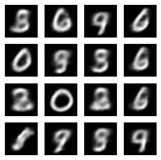
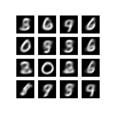
顯示最後一個訓練 epoch 中產生的圖片
def display_image(epoch_no):
  return PIL.Image.open('image_at_epoch_{:04d}.png'.format(epoch_no))
plt.imshow(display_image(epoch))
plt.axis('off')  # Display images
(-0.5, 399.5, 399.5, -0.5)
顯示所有已儲存圖片的動畫 GIF
anim_file = 'cvae.gif'

with imageio.get_writer(anim_file, mode='I') as writer:
  filenames = glob.glob('image*.png')
  filenames = sorted(filenames)
  for filename in filenames:
    image = imageio.imread(filename)
    writer.append_data(image)
  image = imageio.imread(filename)
  writer.append_data(image)
/tmpfs/tmp/ipykernel_129481/1290275450.py:7: DeprecationWarning: Starting with ImageIO v3 the behavior of this function will switch to that of iio.v3.imread. To keep the current behavior (and make this warning disappear) use `import imageio.v2 as imageio` or call `imageio.v2.imread` directly.
  image = imageio.imread(filename)
/tmpfs/tmp/ipykernel_129481/1290275450.py:9: DeprecationWarning: Starting with ImageIO v3 the behavior of this function will switch to that of iio.v3.imread. To keep the current behavior (and make this warning disappear) use `import imageio.v2 as imageio` or call `imageio.v2.imread` directly.
  image = imageio.imread(filename)
import tensorflow_docs.vis.embed as embed
embed.embed_file(anim_file)
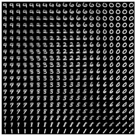
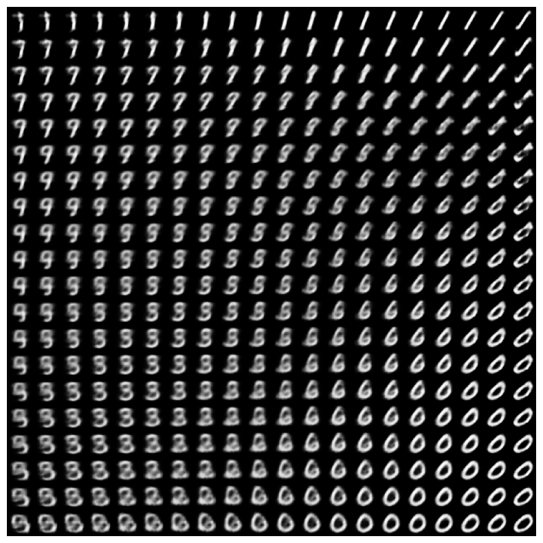
從潛在空間顯示數字的 2D 歧管
執行以下程式碼會顯示不同數字類別的連續分佈,每個數字都會在 2D 潛在空間中變形為另一個數字。使用 TensorFlow Probability 為潛在空間產生標準常態分佈。
def plot_latent_images(model, n, digit_size=28):
  """Plots n x n digit images decoded from the latent space."""

  norm = tfp.distributions.Normal(0, 1)
  grid_x = norm.quantile(np.linspace(0.05, 0.95, n))
  grid_y = norm.quantile(np.linspace(0.05, 0.95, n))
  image_width = digit_size*n
  image_height = image_width
  image = np.zeros((image_height, image_width))

  for i, yi in enumerate(grid_x):
    for j, xi in enumerate(grid_y):
      z = np.array([[xi, yi]])
      x_decoded = model.sample(z)
      digit = tf.reshape(x_decoded[0], (digit_size, digit_size))
      image[i * digit_size: (i + 1) * digit_size,
            j * digit_size: (j + 1) * digit_size] = digit.numpy()

  plt.figure(figsize=(10, 10))
  plt.imshow(image, cmap='Greys_r')
  plt.axis('Off')
  plt.show()
plot_latent_images(model, 20)
後續步驟
本教學課程示範如何使用 TensorFlow 實作卷積變分自動編碼器。
作為後續步驟,您可以嘗試透過增加網路大小來改善模型輸出。例如,您可以嘗試將每個 Conv2D 和 Conv2DTranspose 層的 filter 參數設定為 512。請注意,為了產生最終的 2D 潛在圖片圖,您需要將 latent_dim 保持為 2。此外,訓練時間會隨著網路大小增加而增加。
您也可以嘗試使用不同的資料集 (例如 CIFAR-10) 實作 VAE。
VAE 可以用幾種不同的樣式實作,複雜度也各不相同。您可以在以下來源中找到其他實作方式
如果您想進一步瞭解 VAE 的詳細資訊,請參閱 變分自動編碼器簡介。