
|
|
|
 在 GitHub 上檢視原始碼 在 GitHub 上檢視原始碼
|
|
本教學課程說明如何使用自訂訓練迴圈訓練機器學習模型,以依物種分類企鵝。在本筆記本中,您將使用 TensorFlow 來完成下列事項:
- 匯入資料集
- 建立簡易線性模型
- 訓練模型
- 評估模型的效力
- 使用已訓練的模型進行預測
TensorFlow 程式設計
本教學課程示範下列 TensorFlow 程式設計工作:
- 使用 TensorFlow Datasets API 匯入資料
- 使用 Keras API 建立模型和層
企鵝分類問題
假設您是一位鳥類學家,正在尋找自動化方法來分類您找到的每隻企鵝。機器學習提供許多演算法,可統計方式分類企鵝。例如,精密的機器學習程式可以根據相片分類企鵝。您在本教學課程中建立的模型比較簡單。它根據企鵝的體重、鰭狀肢長度和喙部(特別是其 culmen 的長度和寬度測量值)來分類企鵝。
企鵝共有 18 種,但在本教學課程中,您只會嘗試分類下列三種:
- 帽帶企鵝
- 巴布亞企鵝
- 阿德利企鵝

|
|
圖 1. 帽帶、巴布亞 和 阿德利 企鵝 (Artwork by @allison_horst, CC BY-SA 2.0)。 |
幸運的是,研究團隊已建立並分享了 334 隻企鵝的資料集,其中包含體重、鰭狀肢長度、喙部測量值和其他資料。此資料集也很方便地以 penguins TensorFlow Dataset 的形式提供。
設定
安裝企鵝資料集的 tfds-nightly 套件。tfds-nightly 套件是 TensorFlow Datasets (TFDS) 的每晚發布版本。如需 TFDS 的詳細資訊,請參閱 TensorFlow Datasets 總覽。
pip install -q tfds-nightly
然後從 Colab 選單中選取「Runtime (執行階段) > Restart Runtime (重新啟動執行階段)」,以重新啟動 Colab 執行階段。
在未先重新啟動執行階段的情況下,請勿繼續本教學課程的其餘部分。
匯入 TensorFlow 和其他必要的 Python 模組。
import os
import tensorflow as tf
import tensorflow_datasets as tfds
import matplotlib.pyplot as plt

print("TensorFlow version: {}".format(tf.__version__))
print("TensorFlow Datasets version: ",tfds.__version__)
2023-10-04 01:38:42.243833: E tensorflow/compiler/xla/stream_executor/cuda/cuda_dnn.cc:9342] Unable to register cuDNN factory: Attempting to register factory for plugin cuDNN when one has already been registered
2023-10-04 01:38:42.243876: E tensorflow/compiler/xla/stream_executor/cuda/cuda_fft.cc:609] Unable to register cuFFT factory: Attempting to register factory for plugin cuFFT when one has already been registered
2023-10-04 01:38:42.243916: E tensorflow/compiler/xla/stream_executor/cuda/cuda_blas.cc:1518] Unable to register cuBLAS factory: Attempting to register factory for plugin cuBLAS when one has already been registered
TensorFlow version: 2.14.0
TensorFlow Datasets version:  4.9.3+nightly
匯入資料集
預設的 penguins/processed TensorFlow Dataset 已清理、正規化,並準備好用於建立模型。在您下載已處理的資料之前,請先預覽簡化版本,以熟悉原始企鵝調查資料。
預覽資料
使用 TensorFlow Datasets tfds.load 方法下載簡化版本的企鵝資料集 (penguins/simple)。此資料集中有 344 筆資料記錄。將前五筆記錄擷取到 DataFrame 物件中,以檢查此資料集中值的範例
ds_preview, info = tfds.load('penguins/simple', split='train', with_info=True)
df = tfds.as_dataframe(ds_preview.take(5), info)
print(df)
print(info.features)
2023-10-04 01:38:46.464244: W tensorflow/core/common_runtime/gpu/gpu_device.cc:2211] Cannot dlopen some GPU libraries. Please make sure the missing libraries mentioned above are installed properly if you would like to use GPU. Follow the guide at https://tensorflow.dev.org.tw/install/gpu for how to download and setup the required libraries for your platform.
Skipping registering GPU devices...
body_mass_g  culmen_depth_mm  culmen_length_mm  flipper_length_mm  island  \
0       4200.0             13.9         45.500000              210.0       0
1       4650.0             13.7         40.900002              214.0       0
2       5300.0             14.2         51.299999              218.0       0
3       5650.0             15.0         47.799999              215.0       0
4       5050.0             15.8         46.299999              215.0       0

   sex  species
0    0        2
1    0        2
2    1        2
3    1        2
4    1        2
FeaturesDict({
    'body_mass_g': float32,
    'culmen_depth_mm': float32,
    'culmen_length_mm': float32,
    'flipper_length_mm': float32,
    'island': ClassLabel(shape=(), dtype=int64, num_classes=3),
    'sex': ClassLabel(shape=(), dtype=int64, num_classes=3),
    'species': ClassLabel(shape=(), dtype=int64, num_classes=3),
})
2023-10-04 01:38:46.724179: W tensorflow/core/kernels/data/cache_dataset_ops.cc:854] The calling iterator did not fully read the dataset being cached. In order to avoid unexpected truncation of the dataset, the partially cached contents of the dataset  will be discarded. This can happen if you have an input pipeline similar to `dataset.cache().take(k).repeat()`. You should use `dataset.take(k).cache().repeat()` instead.
編號的列是資料記錄,每行一個範例,其中
在資料集中,企鵝物種的標籤以數字表示,以便在您建立的模型中更易於使用。這些數字對應於下列企鵝物種:
0:阿德利企鵝1:帽帶企鵝2:巴布亞企鵝
建立一個包含依此順序排列的企鵝物種名稱的清單。您將使用此清單來解譯分類模型的輸出
class_names = ['Adélie', 'Chinstrap', 'Gentoo']
如需特徵和標籤的詳細資訊,請參閱機器學習速成課程的「機器學習術語」一節。
下載已預先處理的資料集
現在,使用 tfds.load 方法下載已預先處理的企鵝資料集 (penguins/processed),此方法會傳回 tf.data.Dataset 物件的清單。請注意,penguins/processed 資料集未隨附自己的測試集,因此請使用 80:20 分割來分割完整資料集為訓練集和測試集。稍後您將使用測試資料集來驗證模型。
ds_split, info = tfds.load("penguins/processed", split=['train[:20%]', 'train[20%:]'], as_supervised=True, with_info=True)

ds_test = ds_split[0]
ds_train = ds_split[1]
assert isinstance(ds_test, tf.data.Dataset)

print(info.features)
df_test = tfds.as_dataframe(ds_test.take(5), info)
print("Test dataset sample: ")
print(df_test)

df_train = tfds.as_dataframe(ds_train.take(5), info)
print("Train dataset sample: ")
print(df_train)

ds_train_batch = ds_train.batch(32)
FeaturesDict({
    'features': Tensor(shape=(4,), dtype=float32),
    'species': ClassLabel(shape=(), dtype=int64, num_classes=3),
})
Test dataset sample:
                                         features  species
0  [0.6545454, 0.22619048, 0.89830506, 0.6388889]        2
1        [0.36, 0.04761905, 0.6440678, 0.4027778]        2
2       [0.68, 0.30952382, 0.91525424, 0.6944444]        2
3   [0.6181818, 0.20238096, 0.8135593, 0.6805556]        2
4  [0.5527273, 0.26190478, 0.84745765, 0.7083333]        2
Train dataset sample:
                                         features  species
0  [0.49818182, 0.6904762, 0.42372882, 0.4027778]        0
1      [0.48, 0.071428575, 0.6440678, 0.44444445]        2
2    [0.7236364, 0.9047619, 0.6440678, 0.5833333]        1
3  [0.34545454, 0.5833333, 0.33898306, 0.3472222]        0
4       [0.10909091, 0.75, 0.3559322, 0.41666666]        0
2023-10-04 01:38:47.763232: W tensorflow/core/kernels/data/cache_dataset_ops.cc:854] The calling iterator did not fully read the dataset being cached. In order to avoid unexpected truncation of the dataset, the partially cached contents of the dataset  will be discarded. This can happen if you have an input pipeline similar to `dataset.cache().take(k).repeat()`. You should use `dataset.take(k).cache().repeat()` instead.
2023-10-04 01:38:47.911328: W tensorflow/core/kernels/data/cache_dataset_ops.cc:854] The calling iterator did not fully read the dataset being cached. In order to avoid unexpected truncation of the dataset, the partially cached contents of the dataset  will be discarded. This can happen if you have an input pipeline similar to `dataset.cache().take(k).repeat()`. You should use `dataset.take(k).cache().repeat()` instead.
請注意,此版本的資料集已過處理,方法是將資料縮減為四個標準化特徵和一個物種標籤。採用此格式,資料可以快速用於訓練模型,而無需進一步處理。
features, labels = next(iter(ds_train_batch))

print(features)
print(labels)
tf.Tensor(
[[0.49818182 0.6904762  0.42372882 0.4027778 ]
 [0.48       0.07142857 0.6440678  0.44444445]
 [0.7236364  0.9047619  0.6440678  0.5833333 ]
 [0.34545454 0.5833333  0.33898306 0.3472222 ]
 [0.10909091 0.75       0.3559322  0.41666666]
 [0.6690909  0.63095236 0.47457626 0.19444445]
 [0.8036364  0.9166667  0.4915254  0.44444445]
 [0.4909091  0.75       0.37288135 0.22916667]
 [0.33454546 0.85714287 0.37288135 0.2361111 ]
 [0.32       0.41666666 0.2542373  0.1388889 ]
 [0.41454545 0.5952381  0.5084746  0.19444445]
 [0.14909092 0.48809522 0.2542373  0.125     ]
 [0.23636363 0.4642857  0.27118644 0.05555556]
 [0.22181818 0.5952381  0.22033899 0.3472222 ]
 [0.24727273 0.5595238  0.15254237 0.25694445]
 [0.63272727 0.35714287 0.88135594 0.8194444 ]
 [0.47272727 0.15476191 0.6440678  0.4722222 ]
 [0.6036364  0.23809524 0.84745765 0.7361111 ]
 [0.26909092 0.5595238  0.27118644 0.16666667]
 [0.28       0.71428573 0.20338982 0.5416667 ]
 [0.10545454 0.5714286  0.33898306 0.2847222 ]
 [0.18545455 0.5952381  0.10169491 0.33333334]
 [0.47272727 0.16666667 0.7288136  0.6388889 ]
 [0.45090908 0.1904762  0.7118644  0.5972222 ]
 [0.49454546 0.5        0.3559322  0.25      ]
 [0.6363636  0.22619048 0.7457627  0.5694444 ]
 [0.08727273 0.5952381  0.2542373  0.05555556]
 [0.52       0.22619048 0.7457627  0.5555556 ]
 [0.5090909  0.23809524 0.7288136  0.6666667 ]
 [0.56       0.22619048 0.779661   0.625     ]
 [0.6363636  0.3452381  0.89830506 0.8333333 ]
 [0.15636364 0.47619048 0.20338982 0.04166667]], shape=(32, 4), dtype=float32)
tf.Tensor([0 2 1 0 0 1 1 1 0 1 1 0 0 0 0 2 2 2 0 0 0 0 2 2 1 2 0 2 2 2 2 0], shape=(32,), dtype=int64)
2023-10-04 01:38:48.063769: W tensorflow/core/kernels/data/cache_dataset_ops.cc:854] The calling iterator did not fully read the dataset being cached. In order to avoid unexpected truncation of the dataset, the partially cached contents of the dataset  will be discarded. This can happen if you have an input pipeline similar to `dataset.cache().take(k).repeat()`. You should use `dataset.take(k).cache().repeat()` instead.
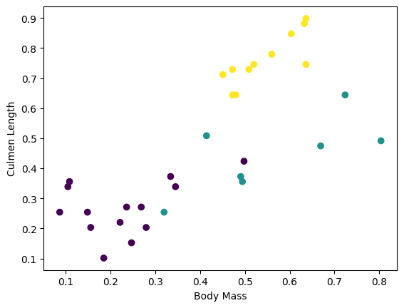
您可以藉由繪製批次中的一些特徵來視覺化一些叢集
plt.scatter(features[:,0],
            features[:,2],
            c=labels,
            cmap='viridis')

plt.xlabel("Body Mass")
plt.ylabel("Culmen Length")
plt.show()
建立簡易線性模型
為何需要模型?
模型是特徵和標籤之間的關係。對於企鵝分類問題,模型定義了體重、鰭狀肢和 culmen 測量值與預測企鵝物種之間的關係。一些簡單的模型可以用幾行代數來描述,但複雜的機器學習模型有大量難以總結的參數。
不使用機器學習,您可以判斷四個特徵與企鵝物種之間的關係嗎?也就是說,您可以使用傳統的程式設計技術 (例如,大量條件陳述式) 來建立模型嗎?也許可以,如果您分析資料集的時間夠長,足以判斷體重和 culmen 測量值與特定物種之間的關係。而在更複雜的資料集上,這會變得困難,甚至不可能。良好的機器學習方法會為您判斷模型。如果您將足夠具代表性的範例饋送到正確的機器學習模型類型,則程式會為您找出關係。
選取模型
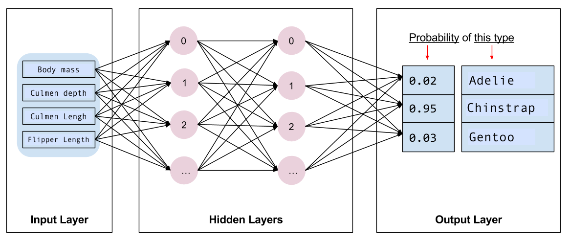
接下來,您需要選取要訓練的模型種類。模型類型有很多種,選取好的模型需要經驗。本教學課程使用神經網路來解決企鵝分類問題。神經網路可以找到特徵和標籤之間的複雜關係。它是一個高度結構化的圖形,組織成一個或多個隱藏層。每個隱藏層都包含一個或多個神經元。神經網路有多個類別,而此程式使用密集或全連線神經網路:一個層中的神經元接收來自前一層中每個神經元的輸入連線。例如,圖 2 說明了一個密集神經網路,其中包含輸入層、兩個隱藏層和一個輸出層
|
|
圖 2. 具有特徵、隱藏層和預測的神經網路。 |
當您從圖 2 訓練模型並將未標記的範例饋送給模型時,它會產生三個預測:此企鵝是給定企鵝物種的可能性。此預測稱為推論。對於此範例,輸出預測的總和為 1.0。在圖 2 中,此預測細分為:阿德利為 0.02,帽帶為 0.95,巴布亞物種為 0.03。這表示模型預測未標記的範例企鵝是帽帶企鵝的機率為 95%。
使用 Keras 建立模型
TensorFlow tf.keras API 是建立模型和圖層的慣用方式。這讓您可以輕鬆建立模型和實驗,同時 Keras 會處理將所有項目連接在一起的複雜性。
tf.keras.Sequential 模型是圖層的線性堆疊。其建構函式接受圖層執行個體的清單,在此案例中為兩個各具有 10 個節點的 tf.keras.layers.Dense 圖層,以及一個具有 3 個節點的輸出圖層,代表您的標籤預測。第一個圖層的 input_shape 參數對應於資料集的特徵數量,而且是必要的
model = tf.keras.Sequential([
  tf.keras.layers.Dense(10, activation=tf.nn.relu, input_shape=(4,)),  # input shape required
  tf.keras.layers.Dense(10, activation=tf.nn.relu),
  tf.keras.layers.Dense(3)
])
啟動函式決定圖層中每個節點的輸出形狀。這些非線性非常重要,如果沒有它們,模型將相當於單一層。有許多 tf.keras.activations,但 ReLU 對於隱藏層很常見。
隱藏層和神經元的理想數量取決於問題和資料集。與機器學習的許多方面一樣,選取神經網路的最佳形狀需要知識和實驗的結合。根據經驗法則,增加隱藏層和神經元的數量通常會建立更強大的模型,這需要更多資料才能有效地訓練。
使用模型
讓我們快速看一下此模型對一批特徵的作用
predictions = model(features)
predictions[:5]
<tf.Tensor: shape=(5, 3), dtype=float32, numpy=
array([[-0.02415227,  0.04778093, -0.54650617],
       [-0.04896604, -0.00673792, -0.49251765],
       [-0.03878566,  0.06066278, -0.78274006],
       [-0.01548526,  0.0427432 , -0.42849454],
       [ 0.01124369,  0.06327108, -0.39197594]], dtype=float32)>
在這裡,每個範例都會傳回每個類別的 logit。
若要將這些 logits 轉換為每個類別的機率,請使用 softmax 函式
tf.nn.softmax(predictions[:5])
<tf.Tensor: shape=(5, 3), dtype=float32, numpy=
array([[0.37485388, 0.4028118 , 0.22233434],
       [0.37245536, 0.38852027, 0.23902439],
       [0.38762808, 0.42815906, 0.18421285],
       [0.36742914, 0.38945913, 0.24311174],
       [0.36743495, 0.38705766, 0.2455073 ]], dtype=float32)>
跨類別取得 tf.math.argmax 可為我們提供預測的類別索引。但是,模型尚未經過訓練,因此這些不是好的預測
print("Prediction: {}".format(tf.math.argmax(predictions, axis=1)))
print("    Labels: {}".format(labels))
Prediction: [1 1 1 1 1 1 1 1 1 1 1 1 1 1 1 1 1 1 1 1 1 1 1 1 1 1 1 1 1 1 1 1]
    Labels: [0 2 1 0 0 1 1 1 0 1 1 0 0 0 0 2 2 2 0 0 0 0 2 2 1 2 0 2 2 2 2 0]
訓練模型
訓練是機器學習的階段,在此階段中,模型會逐步最佳化,或模型會學習資料集。目標是充分了解訓練資料集的結構,以便對看不見的資料進行預測。如果您對訓練資料集了解太多,則預測僅適用於其已看到的資料,並且無法一般化。此問題稱為過度配適,這就像記住答案而不是了解如何解決問題。
企鵝分類問題是監督式機器學習的範例:模型是從包含標籤的範例中訓練而來的。在非監督式機器學習中,範例不包含標籤。相反地,模型通常會在特徵中找到模式。
定義損失和梯度函式
訓練和評估階段都需要計算模型的損失。這會測量模型的預測與所需標籤的偏差程度,換句話說,模型執行效果有多差。您想要最小化或最佳化此值。
您的模型將使用 tf.keras.losses.SparseCategoricalCrossentropy 函式計算其損失,此函式會採用模型的類別機率預測和所需的標籤,並傳回範例的平均損失。
loss_object = tf.keras.losses.SparseCategoricalCrossentropy(from_logits=True)
def loss(model, x, y, training):
  # training=training is needed only if there are layers with different
  # behavior during training versus inference (e.g. Dropout).
  y_ = model(x, training=training)

  return loss_object(y_true=y, y_pred=y_)

l = loss(model, features, labels, training=False)
print("Loss test: {}".format(l))
Loss test: 1.1675868034362793
使用 tf.GradientTape 內容來計算用於最佳化模型的梯度
def grad(model, inputs, targets):
  with tf.GradientTape() as tape:
    loss_value = loss(model, inputs, targets, training=True)
  return loss_value, tape.gradient(loss_value, model.trainable_variables)
建立最佳化工具
最佳化工具會將計算出的梯度套用至模型的參數,以最小化 loss 函式。您可以將損失函式視為彎曲的表面 (請參閱圖 3),而您想要透過四處走動找到其最低點。梯度指向最陡峭上升的方向,因此您將朝相反方向移動並向下移動。透過針對每個批次反覆計算損失和梯度,您將在訓練期間調整模型。模型將逐漸找到權重和偏差的最佳組合,以最小化損失。而且損失越低,模型的預測就越好。
|
|
圖 3. 最佳化演算法在 3D 空間中隨時間視覺化。 (來源:史丹佛大學 CS231n 課程,MIT 授權條款,圖片來源:Alec Radford) |
TensorFlow 有許多最佳化演算法可用於訓練。在本教學課程中,您將使用實作隨機梯度下降 (SGD) 演算法的 tf.keras.optimizers.SGD。learning_rate 參數設定每次迭代下坡的步長大小。此速率是您通常會調整以獲得更好結果的超參數。
使用 學習率 0.01 (在每次訓練迭代中乘以梯度的純量值) 具現化最佳化工具
optimizer = tf.keras.optimizers.SGD(learning_rate=0.01)
然後使用此物件來計算單一步驟最佳化
loss_value, grads = grad(model, features, labels)

print("Step: {}, Initial Loss: {}".format(optimizer.iterations.numpy(),
                                          loss_value.numpy()))

optimizer.apply_gradients(zip(grads, model.trainable_variables))

print("Step: {},         Loss: {}".format(optimizer.iterations.numpy(),
                                          loss(model, features, labels, training=True).numpy()))
Step: 0, Initial Loss: 1.1675868034362793
Step: 1,         Loss: 1.1655302047729492
訓練迴圈
在所有組件都就緒的情況下,模型已準備好進行訓練!訓練迴圈會將資料集範例饋送到模型中,以協助模型做出更好的預測。下列程式碼區塊設定了這些訓練步驟:
- 迭代每個週期。週期是資料集的單次傳遞。
- 在一個週期內,迭代訓練
Dataset中的每個範例,抓取其特徵 (x) 和標籤 (y)。 - 使用範例的特徵,做出預測並將其與標籤進行比較。測量預測的不準確性,並使用它來計算模型的損失和梯度。
- 使用
optimizer更新模型的參數。 - 追蹤一些統計資料以進行視覺化。
- 針對每個週期重複執行。
num_epochs 變數是要在資料集集合上迴圈的次數。在下列程式碼中,num_epochs 設定為 201,這表示此訓練迴圈將執行 201 次。與直覺相反,訓練模型的時間越長,並不保證模型會更好。num_epochs 是您可以調整的超參數。選擇正確的數字通常需要經驗和實驗。
## Note: Rerunning this cell uses the same model parameters

# Keep results for plotting
train_loss_results = []
train_accuracy_results = []

num_epochs = 201

for epoch in range(num_epochs):
  epoch_loss_avg = tf.keras.metrics.Mean()
  epoch_accuracy = tf.keras.metrics.SparseCategoricalAccuracy()

  # Training loop - using batches of 32
  for x, y in ds_train_batch:
    # Optimize the model
    loss_value, grads = grad(model, x, y)
    optimizer.apply_gradients(zip(grads, model.trainable_variables))

    # Track progress
    epoch_loss_avg.update_state(loss_value)  # Add current batch loss
    # Compare predicted label to actual label
    # training=True is needed only if there are layers with different
    # behavior during training versus inference (e.g. Dropout).
    epoch_accuracy.update_state(y, model(x, training=True))

  # End epoch
  train_loss_results.append(epoch_loss_avg.result())
  train_accuracy_results.append(epoch_accuracy.result())

  if epoch % 50 == 0:
    print("Epoch {:03d}: Loss: {:.3f}, Accuracy: {:.3%}".format(epoch,
                                                                epoch_loss_avg.result(),
                                                                epoch_accuracy.result()))
Epoch 000: Loss: 1.161, Accuracy: 26.217%
Epoch 050: Loss: 0.769, Accuracy: 80.524%
Epoch 100: Loss: 0.410, Accuracy: 83.895%
Epoch 150: Loss: 0.275, Accuracy: 92.135%
Epoch 200: Loss: 0.198, Accuracy: 95.880%
或者,您可以使用內建的 Keras Model.fit(ds_train_batch) 方法來訓練模型。
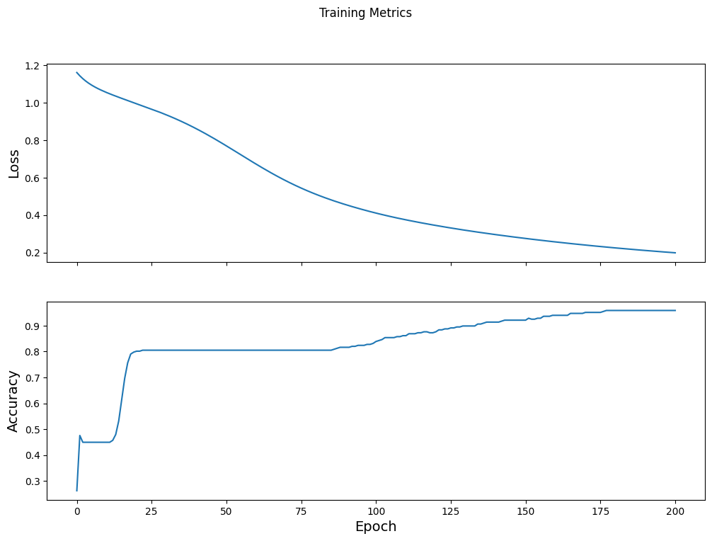
將損失函式隨時間視覺化
雖然列印出模型的訓練進度很有幫助,但您可以使用 TensorBoard (隨 TensorFlow 封裝的可視化和指標工具) 來視覺化進度。對於這個簡單的範例,您將使用 matplotlib 模組建立基本圖表。
解譯這些圖表需要一些經驗,但一般來說,您會希望看到損失減少且準確度提高
fig, axes = plt.subplots(2, sharex=True, figsize=(12, 8))
fig.suptitle('Training Metrics')

axes[0].set_ylabel("Loss", fontsize=14)
axes[0].plot(train_loss_results)

axes[1].set_ylabel("Accuracy", fontsize=14)
axes[1].set_xlabel("Epoch", fontsize=14)
axes[1].plot(train_accuracy_results)
plt.show()
評估模型的效力
現在模型已訓練完成,您可以取得一些關於其效能的統計資料。
評估表示判斷模型進行預測的有效程度。若要判斷模型在企鵝分類方面的有效性,請將一些測量值傳遞給模型,並要求模型預測它們代表的企鵝物種。然後將模型的預測與實際標籤進行比較。例如,在輸入範例中,模型在一半範例中選取了正確的物種,則準確度為 0.5。圖 4 顯示了一個稍微有效的模型,在 5 個預測中獲得 4 個正確的預測,準確度為 80%
| 範例特徵 | 標籤 | 模型預測 | |||
|---|---|---|---|---|---|
| 5.9 | 3.0 | 4.3 | 1.5 | 1 | 1 |
| 6.9 | 3.1 | 5.4 | 2.1 | 2 | 2 |
| 5.1 | 3.3 | 1.7 | 0.5 | 0 | 0 |
| 6.0 | 3.4 | 4.5 | 1.6 | 1 | 2 |
| 5.5 | 2.5 | 4.0 | 1.3 | 1 | 1 |
|
圖 4. 準確度為 80% 的企鵝分類器。 | |||||
設定測試集
評估模型類似於訓練模型。最大的不同之處在於,範例來自個別的測試集,而不是訓練集。為了公平地評估模型的有效性,用於評估模型的範例必須與用於訓練模型的範例不同。
企鵝資料集沒有個別的測試資料集,因此在先前的「下載資料集」一節中,您已將原始資料集分割成測試和訓練資料集。使用 ds_test_batch 資料集進行評估。
在測試資料集上評估模型
與訓練階段不同,模型僅評估測試資料的單一週期。下列程式碼會迭代測試集中的每個範例,並將模型的預測與實際標籤進行比較。此比較用於測量整個測試集上模型的準確度
test_accuracy = tf.keras.metrics.Accuracy()
ds_test_batch = ds_test.batch(10)

for (x, y) in ds_test_batch:
  # training=False is needed only if there are layers with different
  # behavior during training versus inference (e.g. Dropout).
  logits = model(x, training=False)
  prediction = tf.math.argmax(logits, axis=1, output_type=tf.int64)
  test_accuracy(prediction, y)

print("Test set accuracy: {:.3%}".format(test_accuracy.result()))
Test set accuracy: 97.015%
您也可以使用 model.evaluate(ds_test, return_dict=True) keras 函式來取得測試資料集的準確度資訊。
例如,透過檢查最後一批,您可以觀察到模型預測通常是正確的。
tf.stack([y,prediction],axis=1)
<tf.Tensor: shape=(7, 2), dtype=int64, numpy=
array([[1, 1],
       [0, 0],
       [2, 2],
       [0, 0],
       [1, 1],
       [2, 2],
       [0, 0]])>
使用已訓練的模型進行預測
您已訓練模型,並「證明」它在分類企鵝物種方面表現良好 (但並非完美)。現在,讓我們使用已訓練的模型,針對未標記的範例 (也就是包含特徵但不包含標籤的範例) 進行一些預測。
在現實生活中,未標記的範例可能來自許多不同的來源,包括應用程式、CSV 檔案和資料饋送。對於本教學課程,請手動提供三個未標記的範例以預測其標籤。回想一下,標籤數字會對應到具名表示法,如下所示:
0:阿德利企鵝1:帽帶企鵝2:巴布亞企鵝
predict_dataset = tf.convert_to_tensor([
    [0.3, 0.8, 0.4, 0.5,],
    [0.4, 0.1, 0.8, 0.5,],
    [0.7, 0.9, 0.8, 0.4]
])

# training=False is needed only if there are layers with different
# behavior during training versus inference (e.g. Dropout).
predictions = model(predict_dataset, training=False)

for i, logits in enumerate(predictions):
  class_idx = tf.math.argmax(logits).numpy()
  p = tf.nn.softmax(logits)[class_idx]
  name = class_names[class_idx]
  print("Example {} prediction: {} ({:4.1f}%)".format(i, name, 100*p))
Example 0 prediction: Adélie (84.3%)
Example 1 prediction: Gentoo (96.6%)
Example 2 prediction: Chinstrap (86.1%)