
|
|
|
 在 GitHub 上檢視原始碼 在 GitHub 上檢視原始碼
|
|
總覽
使用 TensorFlow Image Summary API,您可以輕鬆記錄張量和任意圖像,並在 TensorBoard 中檢視。這對於取樣和檢查您的輸入資料,或視覺化圖層權重和產生的張量非常有幫助。您也可以將診斷資料記錄為圖像,這在模型開發過程中可能很有幫助。
在本教學課程中,您將學習如何使用 Image Summary API 將張量視覺化為圖像。您也將學習如何取得任意圖像、將其轉換為張量,並在 TensorBoard 中視覺化。您將完成一個簡單但真實的範例,該範例使用 Image Summary 來協助您瞭解模型的效能。
設定
try:
  # %tensorflow_version only exists in Colab.
  %tensorflow_version 2.x
except Exception:
  pass

# Load the TensorBoard notebook extension.
%load_ext tensorboard
TensorFlow 2.x selected.
from datetime import datetime
import io
import itertools
from packaging import version

import tensorflow as tf
from tensorflow import keras

import matplotlib.pyplot as plt
import numpy as np
import sklearn.metrics

print("TensorFlow version: ", tf.__version__)
assert version.parse(tf.__version__).release[0] >= 2, \
    "This notebook requires TensorFlow 2.0 or above."
TensorFlow version: 2.2
下載 Fashion-MNIST 資料集
您將建構一個簡單的神經網路,以對 Fashion-MNIST 資料集中的圖像進行分類。此資料集包含來自 10 個類別的 70,000 張 28x28 灰階時尚產品圖像,每個類別有 7,000 張圖像。
首先,下載資料
# Download the data. The data is already divided into train and test.
# The labels are integers representing classes.
fashion_mnist = keras.datasets.fashion_mnist
(train_images, train_labels), (test_images, test_labels) = \
    fashion_mnist.load_data()

# Names of the integer classes, i.e., 0 -> T-short/top, 1 -> Trouser, etc.
class_names = ['T-shirt/top', 'Trouser', 'Pullover', 'Dress', 'Coat',
    'Sandal', 'Shirt', 'Sneaker', 'Bag', 'Ankle boot']
Downloading data from https://storage.googleapis.com/tensorflow/tf-keras-datasets/train-labels-idx1-ubyte.gz
32768/29515 [=================================] - 0s 0us/step
Downloading data from https://storage.googleapis.com/tensorflow/tf-keras-datasets/train-images-idx3-ubyte.gz
26427392/26421880 [==============================] - 0s 0us/step
Downloading data from https://storage.googleapis.com/tensorflow/tf-keras-datasets/t10k-labels-idx1-ubyte.gz
8192/5148 [===============================================] - 0s 0us/step
Downloading data from https://storage.googleapis.com/tensorflow/tf-keras-datasets/t10k-images-idx3-ubyte.gz
4423680/4422102 [==============================] - 0s 0us/step
視覺化單張圖像
為了瞭解 Image Summary API 的運作方式,您現在將在 TensorBoard 中簡單記錄訓練集中第一張訓練圖像。
在執行此操作之前,請檢查訓練資料的形狀
print("Shape: ", train_images[0].shape)
print("Label: ", train_labels[0], "->", class_names[train_labels[0]])
Shape:  (28, 28)
Label:  9 -> Ankle boot
請注意,資料集中每張圖像的形狀都是形狀為 (28, 28) 的 rank-2 張量,表示高度和寬度。
但是,tf.summary.image() 預期為包含 (batch_size, height, width, channels) 的 rank-4 張量。因此,張量需要重新塑形。
您只記錄一張圖像,因此 batch_size 為 1。圖像為灰階,因此將 channels 設定為 1。
# Reshape the image for the Summary API.
img = np.reshape(train_images[0], (-1, 28, 28, 1))
您現在已準備好記錄此圖像並在 TensorBoard 中檢視它。
# Clear out any prior log data.
!rm -rf logs

# Sets up a timestamped log directory.
logdir = "logs/train_data/" + datetime.now().strftime("%Y%m%d-%H%M%S")
# Creates a file writer for the log directory.
file_writer = tf.summary.create_file_writer(logdir)

# Using the file writer, log the reshaped image.
with file_writer.as_default():
  tf.summary.image("Training data", img, step=0)
現在,使用 TensorBoard 檢查圖像。請稍候幾秒鐘以啟動 UI。
%tensorboard --logdir logs/train_data

「時間序列」儀表板會顯示您剛記錄的圖像。它是「短靴」。
圖像已縮放為預設大小,以便於檢視。如果您想檢視未縮放的原始圖像,請勾選右側「設定」面板底部的「顯示實際圖像大小」。
試用亮度與對比度滑桿,以查看它們如何影響圖像像素。
視覺化多張圖像
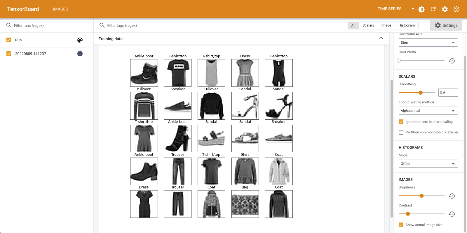
記錄一個張量很棒,但如果您想記錄多個訓練範例呢?
只需在將資料傳遞至 tf.summary.image() 時指定您想要記錄的圖像數量即可。
with file_writer.as_default():
  # Don't forget to reshape.
  images = np.reshape(train_images[0:25], (-1, 28, 28, 1))
  tf.summary.image("25 training data examples", images, max_outputs=25, step=0)

%tensorboard --logdir logs/train_data

記錄任意圖像資料
如果您想視覺化非張量的圖像,例如由 matplotlib 產生的圖像,該怎麼辦?
您需要一些樣板程式碼將繪圖轉換為張量,但在此之後,您就可以開始了。
在下面的程式碼中,您將使用 matplotlib 的 subplot() 函數將前 25 張圖像記錄為美觀的網格。然後,您將在 TensorBoard 中檢視網格
# Clear out prior logging data.
!rm -rf logs/plots

logdir = "logs/plots/" + datetime.now().strftime("%Y%m%d-%H%M%S")
file_writer = tf.summary.create_file_writer(logdir)

def plot_to_image(figure):
  """Converts the matplotlib plot specified by 'figure' to a PNG image and
  returns it. The supplied figure is closed and inaccessible after this call."""
  # Save the plot to a PNG in memory.
  buf = io.BytesIO()
  plt.savefig(buf, format='png')
  # Closing the figure prevents it from being displayed directly inside
  # the notebook.
  plt.close(figure)
  buf.seek(0)
  # Convert PNG buffer to TF image
  image = tf.image.decode_png(buf.getvalue(), channels=4)
  # Add the batch dimension
  image = tf.expand_dims(image, 0)
  return image

def image_grid():
  """Return a 5x5 grid of the MNIST images as a matplotlib figure."""
  # Create a figure to contain the plot.
  figure = plt.figure(figsize=(10,10))
  for i in range(25):
    # Start next subplot.
    plt.subplot(5, 5, i + 1, title=class_names[train_labels[i]])
    plt.xticks([])
    plt.yticks([])
    plt.grid(False)
    plt.imshow(train_images[i], cmap=plt.cm.binary)

  return figure

# Prepare the plot
figure = image_grid()
# Convert to image and log
with file_writer.as_default():
  tf.summary.image("Training data", plot_to_image(figure), step=0)

%tensorboard --logdir logs/plots
建構圖像分類器
現在將所有這些與真實範例結合在一起。畢竟,您來這裡是要進行機器學習,而不是繪製漂亮的圖片!
您將使用圖像摘要來瞭解模型在訓練 Fashion-MNIST 資料集的簡單分類器時的表現。
首先,建立一個非常簡單的模型並編譯它,設定最佳化器和損失函數。編譯步驟也指定您想要記錄分類器的準確度。
model = keras.models.Sequential([
    keras.layers.Flatten(input_shape=(28, 28)),
    keras.layers.Dense(32, activation='relu'),
    keras.layers.Dense(10, activation='softmax')
])

model.compile(
    optimizer='adam',
    loss='sparse_categorical_crossentropy',
    metrics=['accuracy']
)
在訓練分類器時,查看混淆矩陣很有用。混淆矩陣為您提供有關分類器在測試資料上表現的詳細知識。
定義一個計算混淆矩陣的函數。您將使用方便的 Scikit-learn 函數來執行此操作,然後使用 matplotlib 繪製它。
def plot_confusion_matrix(cm, class_names):
  """
  Returns a matplotlib figure containing the plotted confusion matrix.

  Args:
    cm (array, shape = [n, n]): a confusion matrix of integer classes
    class_names (array, shape = [n]): String names of the integer classes
  """
  figure = plt.figure(figsize=(8, 8))
  plt.imshow(cm, interpolation='nearest', cmap=plt.cm.Blues)
  plt.title("Confusion matrix")
  plt.colorbar()
  tick_marks = np.arange(len(class_names))
  plt.xticks(tick_marks, class_names, rotation=45)
  plt.yticks(tick_marks, class_names)

  # Compute the labels from the normalized confusion matrix.
  labels = np.around(cm.astype('float') / cm.sum(axis=1)[:, np.newaxis], decimals=2)

  # Use white text if squares are dark; otherwise black.
  threshold = cm.max() / 2.
  for i, j in itertools.product(range(cm.shape[0]), range(cm.shape[1])):
    color = "white" if cm[i, j] > threshold else "black"
    plt.text(j, i, labels[i, j], horizontalalignment="center", color=color)

  plt.tight_layout()
  plt.ylabel('True label')
  plt.xlabel('Predicted label')
  return figure
您現在已準備好訓練分類器並定期記錄混淆矩陣。
以下是您將執行的操作
- 建立 Keras TensorBoard 回呼以記錄基本指標
- 建立 Keras LambdaCallback 以在每個 epoch 結束時記錄混淆矩陣
- 使用 Model.fit() 訓練模型,確保傳遞兩個回呼
隨著訓練進度,向下捲動以查看 TensorBoard 啟動。
# Clear out prior logging data.
!rm -rf logs/image

logdir = "logs/image/" + datetime.now().strftime("%Y%m%d-%H%M%S")
# Define the basic TensorBoard callback.
tensorboard_callback = keras.callbacks.TensorBoard(log_dir=logdir)
file_writer_cm = tf.summary.create_file_writer(logdir + '/cm')
def log_confusion_matrix(epoch, logs):
  # Use the model to predict the values from the validation dataset.
  test_pred_raw = model.predict(test_images)
  test_pred = np.argmax(test_pred_raw, axis=1)

  # Calculate the confusion matrix.
  cm = sklearn.metrics.confusion_matrix(test_labels, test_pred)
  # Log the confusion matrix as an image summary.
  figure = plot_confusion_matrix(cm, class_names=class_names)
  cm_image = plot_to_image(figure)

  # Log the confusion matrix as an image summary.
  with file_writer_cm.as_default():
    tf.summary.image("epoch_confusion_matrix", cm_image, step=epoch)

# Define the per-epoch callback.
cm_callback = keras.callbacks.LambdaCallback(on_epoch_end=log_confusion_matrix)
# Start TensorBoard.
%tensorboard --logdir logs/image

# Train the classifier.
model.fit(
    train_images,
    train_labels,
    epochs=5,
    verbose=0, # Suppress chatty output
    callbacks=[tensorboard_callback, cm_callback],
    validation_data=(test_images, test_labels),
)
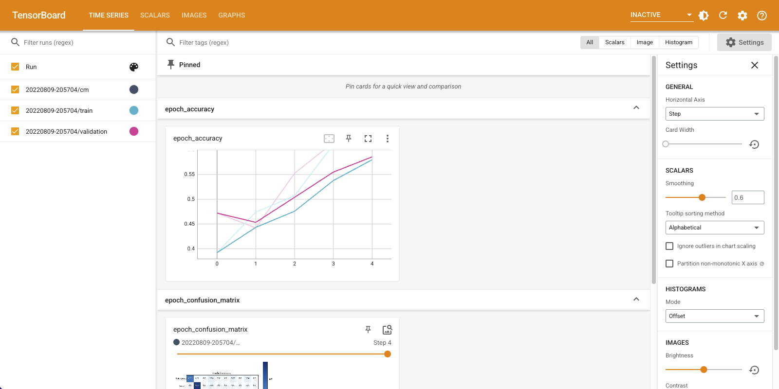
請注意,訓練集和驗證集的準確度都在攀升。這是個好兆頭。但是模型在資料的特定子集上的表現如何?
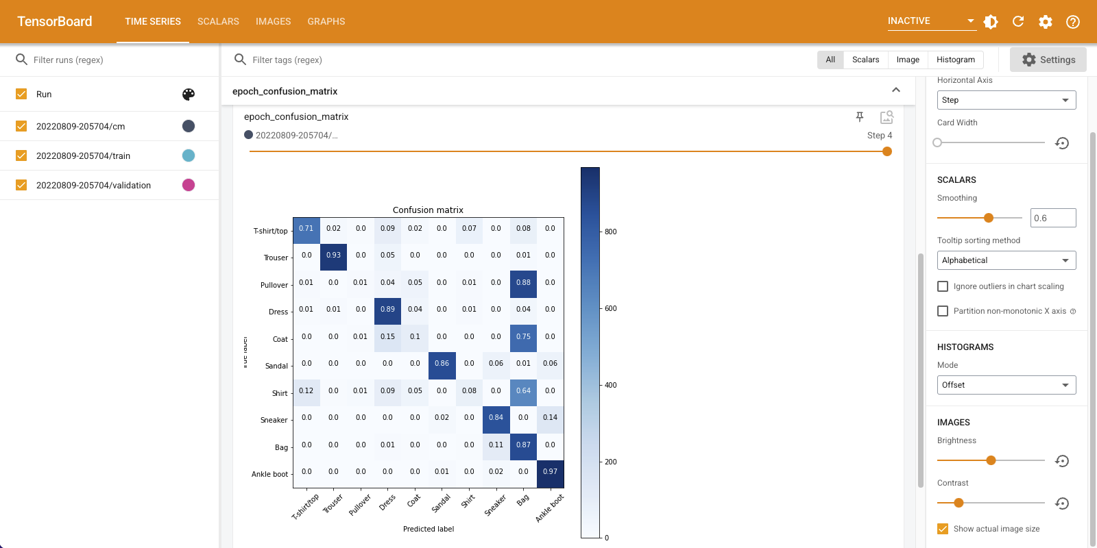
向下捲動「時間序列」儀表板以視覺化您記錄的混淆矩陣。勾選「設定」面板底部的「顯示實際圖像大小」,以完整大小查看混淆矩陣。
預設情況下,儀表板會顯示最後記錄步驟或 epoch 的圖像摘要。使用滑桿檢視先前的混淆矩陣。請注意,隨著訓練進度,矩陣如何顯著變化,沿對角線聚合的較深方塊,以及矩陣的其餘部分如何趨向於 0 和白色。這表示您的分類器正在隨著訓練進度而改進!做得好!
混淆矩陣顯示這個簡單的模型存在一些問題。儘管取得了很大的進展,但襯衫、T 恤和套頭衫彼此混淆。模型需要更多努力。
如果您有興趣,請嘗試使用卷積網路 (CNN) 來改進這個模型。