
|
|
|
 在 GitHub 上檢視 在 GitHub 上檢視
|
|
歡迎使用 TensorFlow 決策樹森林 (TF-DF) 的學習排序 Colab。在此 Colab 中,您將學習如何使用 TF-DF 進行排序。
本 Colab 假設您已熟悉初學者 Colab 中介紹的概念,特別是有關 TF-DF 安裝的部分。
在此 Colab 中,您將:
- 瞭解什麼是排序模型。
- 在 LETOR3 資料集上訓練梯度提升樹模型。
- 評估此模型的品質。
安裝 TensorFlow 決策樹森林
執行下列儲存格來安裝 TF-DF。
pip install tensorflow_decision_forests
需要 Wurlitzer 才能在 Colab 中顯示詳細的訓練記錄 (在模型建構函式中使用 verbose=2 時)。
pip install wurlitzer
匯入程式庫
import os
# Keep using Keras 2
os.environ['TF_USE_LEGACY_KERAS'] = '1'

import tensorflow_decision_forests as tfdf

import numpy as np
import pandas as pd
import tensorflow as tf
import tf_keras
import math
隱藏的程式碼儲存格限制了 Colab 中的輸出高度。
# Check the version of TensorFlow Decision Forests
print("Found TensorFlow Decision Forests v" + tfdf.__version__)
Found TensorFlow Decision Forests v1.9.0
什麼是排序模型?
排序模型的目標是正確排序項目。例如,排序可用於選取使用者查詢後要擷取的最佳文件。
表示排序資料集的常見方法是使用「相關性」分數:元素的順序由其相關性定義:相關性較高的項目應在相關性較低的項目之前。錯誤的成本由預測項目的相關性與正確項目的相關性之間的差異來定義。例如,錯誤排序相關性分別為 3 和 4 的兩個項目不如錯誤排序相關性分別為 1 和 5 的兩個項目那麼糟糕。
TF-DF 期望排序資料集以「平面」格式呈現。查詢和對應文件的資料集可能如下所示:
| 查詢 | 文件 ID | 特徵 1 | 特徵 2 | 相關性 |
|---|---|---|---|---|
| 貓 | 1 | 0.1 | 藍色 | 4 |
| 貓 | 2 | 0.5 | 綠色 | 1 |
| 貓 | 3 | 0.2 | 紅色 | 2 |
| 狗 | 4 | 不適用 | 紅色 | 0 |
| 狗 | 5 | 0.2 | 紅色 | 0 |
| 狗 | 6 | 0.6 | 綠色 | 1 |
相關性/標籤是介於 0 到 5 之間的浮點數值 (通常介於 0 到 4 之間),其中 0 表示「完全不相關」,4 表示「非常相關」,5 表示「與查詢相同」。
在此範例中,文件 1 與查詢「貓」非常相關,而文件 2 僅與貓「相關」。沒有任何文件真正談論「狗」(文件 6 的最高相關性為 1)。但是,狗查詢仍然期望傳回文件 6 (因為這是最「多」談論狗的文件)。
有趣的是,決策樹森林通常是不錯的排序器,並且許多最先進的排序模型都是決策樹森林。
讓我們訓練一個排序模型
在此範例中,使用 LETOR3 資料集的範例。更精確地說,我們想要從 LETOR3 儲存庫下載 OHSUMED.zip。此資料集以 libsvm 格式儲存,因此我們需要將其轉換為 csv。
archive_path = tf_keras.utils.get_file("letor.zip",
  "https://download.microsoft.com/download/E/7/E/E7EABEF1-4C7B-4E31-ACE5-73927950ED5E/Letor.zip",
  extract=True)

# Path to a ranking ataset using libsvm format.
raw_dataset_path = os.path.join(os.path.dirname(archive_path),"OHSUMED/Data/Fold1/trainingset.txt")
Downloading data from https://download.microsoft.com/download/E/7/E/E7EABEF1-4C7B-4E31-ACE5-73927950ED5E/Letor.zip
61824018/61824018 [==============================] - 7s 0us/step
以下是資料集的前幾行
head {raw_dataset_path}
第一步是將此資料集轉換為上述的「平面」格式。
def convert_libsvm_to_csv(src_path, dst_path):
  """Converts a libsvm ranking dataset into a flat csv file.

  Note: This code is specific to the LETOR3 dataset.
  """
  dst_handle = open(dst_path, "w")
  first_line = True
  for src_line in open(src_path,"r"):
    # Note: The last 3 items are comments.
    items = src_line.split(" ")[:-3]
    relevance = items[0]
    group = items[1].split(":")[1]
    features = [ item.split(":") for item in items[2:]]

    if first_line:
      # Csv header
      dst_handle.write("relevance,group," + ",".join(["f_" + feature[0] for feature in features]) + "\n")
      first_line = False
    dst_handle.write(relevance + ",g_" + group + "," + (",".join([feature[1] for feature in features])) + "\n")
  dst_handle.close()

# Convert the dataset.
csv_dataset_path="/tmp/ohsumed.csv"
convert_libsvm_to_csv(raw_dataset_path, csv_dataset_path)

# Load a dataset into a Pandas Dataframe.
dataset_df = pd.read_csv(csv_dataset_path)

# Display the first 3 examples.
dataset_df.head(3)
在此資料集中,每一列代表一對查詢/文件 (稱為「群組」)。「相關性」表示查詢與文件的匹配程度。
查詢和文件的特徵合併在「f1-25」中。特徵的確切定義未知,但它類似於
- 查詢中的字數
- 查詢和文件之間常見的字數
- 查詢的嵌入與文件的嵌入之間的餘弦相似度。
- ...
讓我們將 Pandas Dataframe 轉換為 TensorFlow 資料集
dataset_ds = tfdf.keras.pd_dataframe_to_tf_dataset(dataset_df, label="relevance", task=tfdf.keras.Task.RANKING)
讓我們設定並訓練我們的排序模型。
%set_cell_height 400

model = tfdf.keras.GradientBoostedTreesModel(
    task=tfdf.keras.Task.RANKING,
    ranking_group="group",
    num_trees=50)

model.fit(dataset_ds)
<IPython.core.display.Javascript object>
Warning: The `num_threads` constructor argument is not set and the number of CPU is os.cpu_count()=32 > 32. Setting num_threads to 32. Set num_threads manually to use more than 32 cpus.
WARNING:absl:The `num_threads` constructor argument is not set and the number of CPU is os.cpu_count()=32 > 32. Setting num_threads to 32. Set num_threads manually to use more than 32 cpus.
Use /tmpfs/tmp/tmpzqjjgty3 as temporary training directory
Reading training dataset...
[WARNING 24-04-20 11:09:14.5069 UTC gradient_boosted_trees.cc:1840] "goss_alpha" set but "sampling_method" not equal to "GOSS".
[WARNING 24-04-20 11:09:14.5069 UTC gradient_boosted_trees.cc:1851] "goss_beta" set but "sampling_method" not equal to "GOSS".
[WARNING 24-04-20 11:09:14.5069 UTC gradient_boosted_trees.cc:1865] "selective_gradient_boosting_ratio" set but "sampling_method" not equal to "SELGB".
Training dataset read in 0:00:03.986733. Found 9219 examples.
Training model...
Model trained in 0:00:00.757738
Compiling model...
[INFO 24-04-20 11:09:19.2736 UTC kernel.cc:1233] Loading model from path /tmpfs/tmp/tmpzqjjgty3/model/ with prefix fa7585ffd7c24e56
[INFO 24-04-20 11:09:19.2748 UTC quick_scorer_extended.cc:911] The binary was compiled without AVX2 support, but your CPU supports it. Enable it for faster model inference.
[INFO 24-04-20 11:09:19.2749 UTC abstract_model.cc:1344] Engine "GradientBoostedTreesQuickScorerExtended" built
[INFO 24-04-20 11:09:19.2749 UTC kernel.cc:1061] Use fast generic engine
Model compiled.
<tf_keras.src.callbacks.History at 0x7fb6979cc8b0>
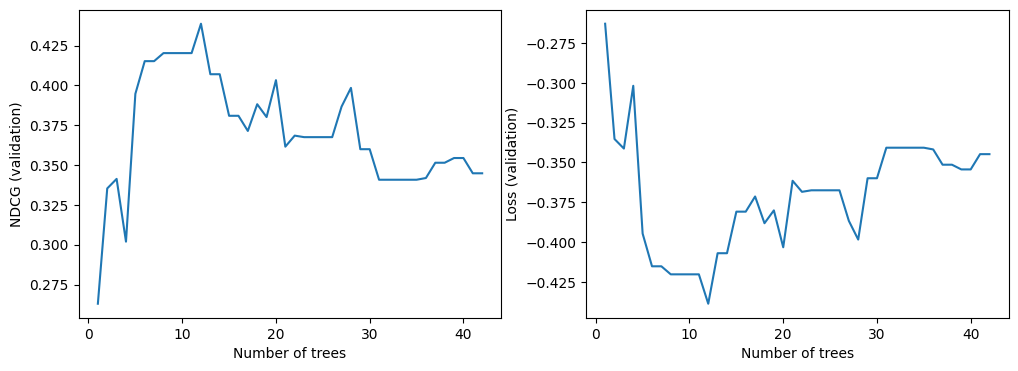
我們現在可以查看模型在驗證資料集上的品質。預設情況下,TF-DF 訓練排序模型以最佳化 NDCG。NDCG 的值介於 0 和 1 之間,其中 1 是完美分數。因此,-NDCG 是模型損失。
import matplotlib.pyplot as plt

logs = model.make_inspector().training_logs()

plt.figure(figsize=(12, 4))

plt.subplot(1, 2, 1)
plt.plot([log.num_trees for log in logs], [log.evaluation.ndcg for log in logs])
plt.xlabel("Number of trees")
plt.ylabel("NDCG (validation)")

plt.subplot(1, 2, 2)
plt.plot([log.num_trees for log in logs], [log.evaluation.loss for log in logs])
plt.xlabel("Number of trees")
plt.ylabel("Loss (validation)")

plt.show()
對於所有 TF-DF 模型,您也可以查看模型報告 (注意:模型報告也包含訓練記錄)
%set_cell_height 400
model.summary()
<IPython.core.display.Javascript object>
Model: "gradient_boosted_trees_model"
_________________________________________________________________
 Layer (type)                Output Shape              Param #
=================================================================
=================================================================
Total params: 1 (1.00 Byte)
Trainable params: 0 (0.00 Byte)
Non-trainable params: 1 (1.00 Byte)
_________________________________________________________________
Type: "GRADIENT_BOOSTED_TREES"
Task: RANKING
Label: "__LABEL"
Rank group: "group"

Input Features (25):
    f_1
    f_10
    f_11
    f_12
    f_13
    f_14
    f_15
    f_16
    f_17
    f_18
    f_19
    f_2
    f_20
    f_21
    f_22
    f_23
    f_24
    f_25
    f_3
    f_4
    f_5
    f_6
    f_7
    f_8
    f_9

No weights

Variable Importance: INV_MEAN_MIN_DEPTH:

    1.  "f_9"  0.326164 ################
    2.  "f_3"  0.318071 ###############
    3.  "f_8"  0.308922 #############
    4.  "f_4"  0.271175 #########
    5. "f_19"  0.221570 ###
    6. "f_10"  0.215666 ##
    7. "f_11"  0.206509 #
    8. "f_22"  0.204742 #
    9. "f_25"  0.204497 #
   10. "f_23"  0.203238
   11. "f_21"  0.200830
   12. "f_24"  0.200445
   13. "f_12"  0.198840
   14. "f_18"  0.197676
   15. "f_20"  0.196634
   16.  "f_6"  0.196085
   17. "f_16"  0.196061
   18.  "f_2"  0.195683
   19.  "f_5"  0.195683
   20. "f_13"  0.195559
   21. "f_17"  0.195559

Variable Importance: NUM_AS_ROOT:

    1. "f_3"  4.000000 ################
    2. "f_4"  4.000000 ################
    3. "f_8"  3.000000 ##########
    4. "f_9"  1.000000

Variable Importance: NUM_NODES:

    1.  "f_8" 25.000000 ################
    2. "f_19" 18.000000 ###########
    3. "f_10" 15.000000 #########
    4.  "f_9" 14.000000 ########
    5.  "f_3" 13.000000 ########
    6. "f_23"  7.000000 ####
    7. "f_24"  6.000000 ###
    8. "f_11"  5.000000 ##
    9. "f_21"  5.000000 ##
   10. "f_25"  5.000000 ##
   11.  "f_4"  5.000000 ##
   12. "f_22"  4.000000 ##
   13. "f_12"  3.000000 #
   14. "f_20"  3.000000 #
   15. "f_16"  2.000000
   16.  "f_6"  2.000000
   17. "f_13"  1.000000
   18. "f_17"  1.000000
   19. "f_18"  1.000000
   20.  "f_2"  1.000000
   21.  "f_5"  1.000000

Variable Importance: SUM_SCORE:

    1.  "f_8" 10779.340861 ################
    2.  "f_9" 8831.772410 #############
    3.  "f_3" 4526.101184 ######
    4.  "f_4" 4360.245403 ######
    5. "f_19" 2325.288894 ###
    6. "f_10" 1881.848369 ##
    7. "f_21" 1674.980191 ##
    8. "f_11" 1127.632256 #
    9. "f_23" 1021.834252 #
   10. "f_24" 914.851512 #
   11. "f_22" 885.619576 #
   12. "f_25" 748.665007 #
   13. "f_20" 310.610858
   14. "f_16" 298.972842
   15.  "f_6" 212.376573
   16. "f_12" 130.725240
   17.  "f_2" 112.124991
   18. "f_18" 86.341193
   19.  "f_5" 65.103908
   20. "f_13" 57.966947
   21. "f_17" 21.930388


Loss: LAMBDA_MART_NDCG5
Validation loss value: -0.438692
Number of trees per iteration: 1
Node format: NOT_SET
Number of trees: 12
Total number of nodes: 286

Number of nodes by tree:
Count: 12 Average: 23.8333 StdDev: 3.50793
Min: 17 Max: 29 Ignored: 0
----------------------------------------------
[ 17, 18) 1   8.33%   8.33% ###
[ 18, 19) 0   0.00%   8.33%
[ 19, 20) 1   8.33%  16.67% ###
[ 20, 21) 0   0.00%  16.67%
[ 21, 22) 2  16.67%  33.33% #######
[ 22, 23) 0   0.00%  33.33%
[ 23, 24) 1   8.33%  41.67% ###
[ 24, 25) 0   0.00%  41.67%
[ 25, 26) 3  25.00%  66.67% ##########
[ 26, 27) 0   0.00%  66.67%
[ 27, 28) 3  25.00%  91.67% ##########
[ 28, 29) 0   0.00%  91.67%
[ 29, 29] 1   8.33% 100.00% ###

Depth by leafs:
Count: 149 Average: 4.14094 StdDev: 1.08696
Min: 1 Max: 5 Ignored: 0
----------------------------------------------
[ 1, 2)  2   1.34%   1.34%
[ 2, 3) 18  12.08%  13.42% ##
[ 3, 4) 13   8.72%  22.15% ##
[ 4, 5) 40  26.85%  48.99% #####
[ 5, 5] 76  51.01% 100.00% ##########

Number of training obs by leaf:
Count: 149 Average: 673.691 StdDev: 2015.44
Min: 5 Max: 8211 Ignored: 0
----------------------------------------------
[    5,  415) 127  85.23%  85.23% ##########
[  415,  825)   6   4.03%  89.26%
[  825, 1236)   2   1.34%  90.60%
[ 1236, 1646)   0   0.00%  90.60%
[ 1646, 2056)   0   0.00%  90.60%
[ 2056, 2467)   1   0.67%  91.28%
[ 2467, 2877)   0   0.00%  91.28%
[ 2877, 3287)   0   0.00%  91.28%
[ 3287, 3698)   1   0.67%  91.95%
[ 3698, 4108)   0   0.00%  91.95%
[ 4108, 4518)   0   0.00%  91.95%
[ 4518, 4929)   1   0.67%  92.62%
[ 4929, 5339)   0   0.00%  92.62%
[ 5339, 5749)   0   0.00%  92.62%
[ 5749, 6160)   1   0.67%  93.29%
[ 6160, 6570)   0   0.00%  93.29%
[ 6570, 6980)   0   0.00%  93.29%
[ 6980, 7391)   0   0.00%  93.29%
[ 7391, 7801)   8   5.37%  98.66% #
[ 7801, 8211]   2   1.34% 100.00%

Attribute in nodes:
    25 : f_8 [NUMERICAL]
    18 : f_19 [NUMERICAL]
    15 : f_10 [NUMERICAL]
    14 : f_9 [NUMERICAL]
    13 : f_3 [NUMERICAL]
    7 : f_23 [NUMERICAL]
    6 : f_24 [NUMERICAL]
    5 : f_4 [NUMERICAL]
    5 : f_25 [NUMERICAL]
    5 : f_21 [NUMERICAL]
    5 : f_11 [NUMERICAL]
    4 : f_22 [NUMERICAL]
    3 : f_20 [NUMERICAL]
    3 : f_12 [NUMERICAL]
    2 : f_6 [NUMERICAL]
    2 : f_16 [NUMERICAL]
    1 : f_5 [NUMERICAL]
    1 : f_2 [NUMERICAL]
    1 : f_18 [NUMERICAL]
    1 : f_17 [NUMERICAL]
    1 : f_13 [NUMERICAL]

Attribute in nodes with depth <= 0:
    4 : f_4 [NUMERICAL]
    4 : f_3 [NUMERICAL]
    3 : f_8 [NUMERICAL]
    1 : f_9 [NUMERICAL]

Attribute in nodes with depth <= 1:
    11 : f_9 [NUMERICAL]
    9 : f_8 [NUMERICAL]
    4 : f_4 [NUMERICAL]
    4 : f_3 [NUMERICAL]
    1 : f_25 [NUMERICAL]
    1 : f_24 [NUMERICAL]
    1 : f_23 [NUMERICAL]
    1 : f_22 [NUMERICAL]
    1 : f_19 [NUMERICAL]
    1 : f_11 [NUMERICAL]

Attribute in nodes with depth <= 2:
    15 : f_8 [NUMERICAL]
    12 : f_9 [NUMERICAL]
    11 : f_3 [NUMERICAL]
    6 : f_19 [NUMERICAL]
    5 : f_4 [NUMERICAL]
    2 : f_25 [NUMERICAL]
    2 : f_11 [NUMERICAL]
    2 : f_10 [NUMERICAL]
    1 : f_24 [NUMERICAL]
    1 : f_23 [NUMERICAL]
    1 : f_22 [NUMERICAL]
    1 : f_18 [NUMERICAL]
    1 : f_17 [NUMERICAL]

Attribute in nodes with depth <= 3:
    22 : f_8 [NUMERICAL]
    13 : f_9 [NUMERICAL]
    11 : f_3 [NUMERICAL]
    10 : f_19 [NUMERICAL]
    9 : f_10 [NUMERICAL]
    5 : f_4 [NUMERICAL]
    5 : f_23 [NUMERICAL]
    5 : f_11 [NUMERICAL]
    4 : f_25 [NUMERICAL]
    4 : f_22 [NUMERICAL]
    4 : f_21 [NUMERICAL]
    3 : f_24 [NUMERICAL]
    2 : f_12 [NUMERICAL]
    1 : f_18 [NUMERICAL]
    1 : f_17 [NUMERICAL]

Attribute in nodes with depth <= 5:
    25 : f_8 [NUMERICAL]
    18 : f_19 [NUMERICAL]
    15 : f_10 [NUMERICAL]
    14 : f_9 [NUMERICAL]
    13 : f_3 [NUMERICAL]
    7 : f_23 [NUMERICAL]
    6 : f_24 [NUMERICAL]
    5 : f_4 [NUMERICAL]
    5 : f_25 [NUMERICAL]
    5 : f_21 [NUMERICAL]
    5 : f_11 [NUMERICAL]
    4 : f_22 [NUMERICAL]
    3 : f_20 [NUMERICAL]
    3 : f_12 [NUMERICAL]
    2 : f_6 [NUMERICAL]
    2 : f_16 [NUMERICAL]
    1 : f_5 [NUMERICAL]
    1 : f_2 [NUMERICAL]
    1 : f_18 [NUMERICAL]
    1 : f_17 [NUMERICAL]
    1 : f_13 [NUMERICAL]

Condition type in nodes:
    137 : HigherCondition
Condition type in nodes with depth <= 0:
    12 : HigherCondition
Condition type in nodes with depth <= 1:
    34 : HigherCondition
Condition type in nodes with depth <= 2:
    60 : HigherCondition
Condition type in nodes with depth <= 3:
    99 : HigherCondition
Condition type in nodes with depth <= 5:
    137 : HigherCondition

Training logs:
Number of iteration to final model: 12
    Iter:1 train-loss:-0.346669 valid-loss:-0.262935  train-NDCG@5:0.346669 valid-NDCG@5:0.262935
    Iter:2 train-loss:-0.412635 valid-loss:-0.335301  train-NDCG@5:0.412635 valid-NDCG@5:0.335301
    Iter:3 train-loss:-0.468270 valid-loss:-0.341295  train-NDCG@5:0.468270 valid-NDCG@5:0.341295
    Iter:4 train-loss:-0.481511 valid-loss:-0.301897  train-NDCG@5:0.481511 valid-NDCG@5:0.301897
    Iter:5 train-loss:-0.473165 valid-loss:-0.394670  train-NDCG@5:0.473165 valid-NDCG@5:0.394670
    Iter:6 train-loss:-0.496260 valid-loss:-0.415201  train-NDCG@5:0.496260 valid-NDCG@5:0.415201
    Iter:16 train-loss:-0.526791 valid-loss:-0.380900  train-NDCG@5:0.526791 valid-NDCG@5:0.380900
    Iter:26 train-loss:-0.560398 valid-loss:-0.367496  train-NDCG@5:0.560398 valid-NDCG@5:0.367496
    Iter:36 train-loss:-0.584252 valid-loss:-0.341845  train-NDCG@5:0.584252 valid-NDCG@5:0.341845
如果您好奇,也可以繪製模型
tfdf.model_plotter.plot_model_in_colab(model, tree_idx=0, max_depth=3)
使用排序模型進行預測
對於傳入的查詢,我們可以使用排序模型來預測一堆文件的相關性。實際上,這表示對於每個查詢,我們都必須提出一組可能與查詢相關或不相關的文件。我們將這些文件稱為候選文件。對於每對查詢/候選文件,我們可以計算訓練期間使用的相同特徵。這是我們的服務資料集。
回到本教學課程開頭的範例,服務資料集可能如下所示:
| 查詢 | 文件 ID | 特徵 1 | 特徵 2 |
|---|---|---|---|
| 魚 | 32 | 0.3 | 藍色 |
| 魚 | 33 | 1.0 | 綠色 |
| 魚 | 34 | 0.4 | 藍色 |
| 魚 | 35 | 不適用 | 棕色 |
請注意,相關性不是服務資料集的一部分,因為這是模型嘗試預測的內容。
服務資料集會饋送到 TF-DF 模型,並為每個文件指派相關性分數。
| 查詢 | 文件 ID | 特徵 1 | 特徵 2 | 相關性 |
|---|---|---|---|---|
| 魚 | 32 | 0.3 | 藍色 | 0.325 |
| 魚 | 33 | 1.0 | 綠色 | 0.125 |
| 魚 | 34 | 0.4 | 藍色 | 0.155 |
| 魚 | 35 | 不適用 | 棕色 | 0.593 |
這表示文件 ID 為 35 的文件預測為與查詢「魚」最相關。
讓我們嘗試使用我們的實際模型來執行此操作。
# Path to a test dataset using libsvm format.
test_dataset_path = os.path.join(os.path.dirname(archive_path),"OHSUMED/Data/Fold1/testset.txt")
# Convert the dataset.
csv_test_dataset_path="/tmp/ohsumed_test.csv"
convert_libsvm_to_csv(raw_dataset_path, csv_test_dataset_path)

# Load a dataset into a Pandas Dataframe.
test_dataset_df = pd.read_csv(csv_test_dataset_path)

# Display the first 3 examples.
test_dataset_df.head(3)
假設我們的查詢是「g_5」,並且測試資料集已包含此查詢的候選文件。
# Filter by "g_5"
serving_dataset_df = test_dataset_df[test_dataset_df['group'] == 'g_5']
# Remove the columns for group and relevance, not needed for predictions.
serving_dataset_df = serving_dataset_df.drop(['relevance', 'group'], axis=1)
# Convert to a Tensorflow dataset
serving_dataset_ds = tfdf.keras.pd_dataframe_to_tf_dataset(serving_dataset_df, task=tfdf.keras.Task.RANKING)
# Run predictions with on all candidate documents
predictions = model.predict(serving_dataset_ds)
1/1 [==============================] - 0s 176ms/step
我們可以使用新增預測到資料框架,並使用它們來尋找得分最高的文件。
serving_dataset_df['prediction_score'] = predictions
serving_dataset_df.sort_values(by=['prediction_score'], ascending=False).head()