鄰近性和原型與隨機森林

在 TensorFlow.org 上檢視

在 Google Colab 中執行

在 GitHub 上檢視

下載筆記本

簡介

Leo Breiman 是 隨機森林 學習演算法的作者，他提出了一種方法來測量兩個範例之間使用預先訓練的隨機森林 (RF) 模型的鄰近性（也稱為相似性）。他將此方法評定為「[...] 隨機森林中最有用的工具之一」。在本筆記本中，我們實作此方法並展示如何使用它來解讀模型。

此筆記本是使用 TensorFlow 決策樹森林 程式庫實作的。如果您熟悉初學者 Colab 的內容，就更容易理解此文件。

鄰近性

兩個範例之間的鄰近性（或相似性）是一個數字，表示這兩個範例有多「接近」。以下是範例 \(\{e_1, e_2, e_3\}\) 之間相似性的範例

\[ \mathrm{proxy}(e_1, e_2) = 0.1 \\ \mathrm{proxy}(e_2, e_3) = 9.6 \\ \mathrm{proxy}(e_3, e_1) = 4.1 \\ \]

為了方便起見，範例之間的鄰近性以矩陣形式表示

	\(e_1\)	\(e_2\)	\(e_3\)
\(e_1\)	\(\mathrm{proxy}(e_1, e_1)\)	\(\mathrm{proxy}(e_1, e_2)\)	\(\mathrm{proxy}(e_1, e_3)\)
\(e_2\)	\(\mathrm{proxy}(e_2, e_1)\)	\(\mathrm{proxy}(e_2, e_2)\)	\(\mathrm{proxy}(e_2, e_3)\)
\(e_3\)	\(\mathrm{proxy}(e_3, e_1)\)	\(\mathrm{proxy}(e_3, e_2)\)	\(\mathrm{proxy}(e_3, e_3)\)

鄰近性用於多種資料分析技術，包括分群、降維或最近鄰分析。因此，它是模型和預測解讀的絕佳工具。

不幸的是，測量兩個表格範例之間的鄰近性並不簡單，因為不同的欄位可能描述不同的數量。例如，嘗試定義以下範例之間的鄰近性。

物種	重量	腿數	年齡	性別
貓	2 公斤	4	2 歲	雄性
狗	6 公斤	4	12 歲	雌性
蜘蛛	5 克	8	3 週	雌性

若要定義上表兩列之間的相似性，您需要指定體重差異與腿數差異或年齡差異的比較程度。此外，關係可能是非線性的，或以其他欄位為條件。例如，狗比蜘蛛活得更久，因此，蜘蛛一年的差異可能不應與狗的一年年齡相同。

Breiman 的鄰近性並非手動定義這些關係，而是將隨機森林模型（我們知道如何在表格資料集上訓練）轉變為鄰近性指標。

隨機森林的鄰近性

隨機森林是決策樹的集合。隨機森林的預測是個別樹狀結構預測的彙總。決策樹的預測是透過根據節點條件將範例從根節點路由到其中一個葉節點來計算的。範例 \(i\) 在樹狀結構 \(t\) 中到達的葉節點稱為其活動葉節點，並記為 \(\mathrm{leaf}(i,t)\)

Breiman 將兩個範例之間的鄰近性定義為這兩個範例之間共享的活動葉節點的比率。形式上，範例 \(i\) 和範例 \(j\) 之間的鄰近性為

\[ \mathrm{prox}(i,j) = \mathrm{prox}(j,i) = \frac{1}{|\mathrm{Trees}|} \sum_{t \in \mathrm{Trees} } \left[ \mathrm{leaf}(i,t) = \mathrm{leaf}(j,t) \right] \]

其中 \(\mathrm{leaf}(j,t)\) 是範例 \(j\) 在樹狀結構 \(t\) 中的活動葉節點索引。

非正式地說，如果兩個範例經常路由到相同的葉節點（即這兩個範例具有相同的活動葉節點），則這些範例是相似的。

讓我們實作此鄰近性函數並在一些範例中使用它。

設定

# Install TensorFlow Dececision Forests and the dependencies used in this colab.
pip install tensorflow_decision_forests plotly scikit-learn wurlitzer -U -qq

import tensorflow_decision_forests as tfdf

import matplotlib.colors as mcolors
import math
import os
import numpy as np
import pandas as pd
from sklearn.manifold import TSNE
import matplotlib.pyplot as plt
from plotly.offline import iplot
import plotly.graph_objs as go

訓練隨機森林模型

此方法依賴於預先訓練的隨機森林模型。首先，我們在 TensorFlow 決策樹森林程式庫 上使用 Adult 二元分類資料集訓練隨機森林模型。Adult 資料集非常適合此範例，因為它包含的欄位沒有自然的比較方式。

# Download a copy of the adult dataset.
wget -q https://raw.githubusercontent.com/google/yggdrasil-decision-forests/main/yggdrasil_decision_forests/test_data/dataset/adult_train.csv -O /tmp/adult_train.csv
wget -q https://raw.githubusercontent.com/google/yggdrasil-decision-forests/main/yggdrasil_decision_forests/test_data/dataset/adult_test.csv -O /tmp/adult_test.csv

# Load the dataset in memory
train_df = pd.read_csv("/tmp/adult_train.csv")
test_df = pd.read_csv("/tmp/adult_test.csv")

# , and convert it into a TensorFlow dataset.
train_ds = tfdf.keras.pd_dataframe_to_tf_dataset(train_df, label="income")
test_ds = tfdf.keras.pd_dataframe_to_tf_dataset(test_df, label="income")

以下是訓練資料集的前五個範例。請注意，不同的欄位代表不同的數量。例如，您將如何比較關係和年齡之間的距離？

# Print the first 5 examples.
train_df.head()

隨機森林訓練如下

# Train a Random Forest
model = tfdf.keras.RandomForestModel(num_trees=1000)
model.fit(train_ds)

Warning: The `num_threads` constructor argument is not set and the number of CPU is os.cpu_count()=32 > 32. Setting num_threads to 32. Set num_threads manually to use more than 32 cpus.
WARNING:absl:The `num_threads` constructor argument is not set and the number of CPU is os.cpu_count()=32 > 32. Setting num_threads to 32. Set num_threads manually to use more than 32 cpus.
Use /tmpfs/tmp/tmpznja9qk8 as temporary training directory
Reading training dataset...
Training dataset read in 0:00:03.886835. Found 22792 examples.
Training model...
[INFO 24-04-20 11:30:19.2658 UTC kernel.cc:1233] Loading model from path /tmpfs/tmp/tmpznja9qk8/model/ with prefix a872f3db44424bcd
[INFO 24-04-20 11:30:23.3606 UTC decision_forest.cc:734] Model loaded with 1000 root(s), 1262362 node(s), and 14 input feature(s).
[INFO 24-04-20 11:30:23.3607 UTC abstract_model.cc:1344] Engine "RandomForestGeneric" built
[INFO 24-04-20 11:30:23.3607 UTC kernel.cc:1061] Use fast generic engine
Model trained in 0:00:09.781512
Compiling model...
Model compiled.
<tf_keras.src.callbacks.History at 0x7f421086a9d0>

隨機森林模型的效能為

model_inspector = model.make_inspector()
out_of_bag_accuracy = model_inspector.evaluation().accuracy
print(f"Out-of-bag accuracy: {out_of_bag_accuracy:.4f}")

Out-of-bag accuracy: 0.8653

這是此資料集上隨機森林模型的預期準確度值。它表示模型已正確訓練。

我們也可以測量模型在測試資料集上的準確度

# The test accuracy is measured on the test datasets.
model.compile(["accuracy"])
test_accuracy = model.evaluate(test_ds, return_dict=True, verbose=0)["accuracy"]
print(f"Test accuracy: {test_accuracy:.4f}")

Test accuracy: 0.8663

鄰近性

首先，我們檢查模型中的樹狀結構數量和測試資料集中的範例數量。

print("The model contains", model_inspector.num_trees(), "trees.")
print("The test dataset contains", test_df.shape[0], "examples.")

The model contains 1000 trees.
The test dataset contains 9769 examples.

predict_get_leaves() 方法會傳回每個範例和每個樹狀結構的活動葉節點索引。

leaves = model.predict_get_leaves(test_ds)
print("The leaf indices:\n", leaves)

[INFO 24-04-20 11:30:34.6052 UTC kernel.cc:1233] Loading model from path /tmpfs/tmp/tmpznja9qk8/model/ with prefix a872f3db44424bcd
[INFO 24-04-20 11:30:37.8796 UTC kernel.cc:1079] Use slow generic engine
WARNING:tensorflow:AutoGraph could not transform <function simple_ml_inference_leaf_index_op_with_handle at 0x7f40ecacf550> and will run it as-is.
Please report this to the TensorFlow team. When filing the bug, set the verbosity to 10 (on Linux, `export AUTOGRAPH_VERBOSITY=10`) and attach the full output.
Cause: could not get source code
To silence this warning, decorate the function with @tf.autograph.experimental.do_not_convert
WARNING:tensorflow:AutoGraph could not transform <function simple_ml_inference_leaf_index_op_with_handle at 0x7f40ecacf550> and will run it as-is.
Please report this to the TensorFlow team. When filing the bug, set the verbosity to 10 (on Linux, `export AUTOGRAPH_VERBOSITY=10`) and attach the full output.
Cause: could not get source code
To silence this warning, decorate the function with @tf.autograph.experimental.do_not_convert
WARNING: AutoGraph could not transform <function simple_ml_inference_leaf_index_op_with_handle at 0x7f40ecacf550> and will run it as-is.
Please report this to the TensorFlow team. When filing the bug, set the verbosity to 10 (on Linux, `export AUTOGRAPH_VERBOSITY=10`) and attach the full output.
Cause: could not get source code
To silence this warning, decorate the function with @tf.autograph.experimental.do_not_convert
The leaf indices:
 [[498 193 142 ... 457 221 198]
 [399 466 423 ... 288 420 444]
 [639 651 562 ... 608 636 625]
 ...
 [149 296 258 ... 153 310 316]
 [481 186 131 ... 432 192 153]
 [  9   0  28 ...   4   1  42]]
2024-04-20 11:30:49.070709: W tensorflow/core/framework/local_rendezvous.cc:404] Local rendezvous is aborting with status: OUT_OF_RANGE: End of sequence

print("The predicted leaves have shape", leaves.shape,
      "(we expect [num_examples, num_trees]")

The predicted leaves have shape (9769, 1000) (we expect [num_examples, num_trees]

在此，leaves[i,j] 是第 j 個樹狀結構中第 i 個範例的活動葉節點索引。

接下來，我們實作先前定義的 \(\mathrm{prox}\) 方程式。

def compute_proximity(leaves, step_size=100):
  """Computes the proximity between each pair of examples.

  Args:
    leaves: A matrix of shape [num_example, num_tree] where the value [i,j] is
      the index of the leaf reached by example "i" in the tree "j".
    step_size: Size of the block of examples for the computation of the
      proximity. Does not impact the results.

  Returns:
    The example pair-wise proximity matrix of shape [n,n] with "n" the number of
    examples.
  """

  example_idx = 0
  num_examples = leaves.shape[0]
  t_leaves = np.transpose(leaves)
  proximities = []

  # Instead of computing the proximity in between all the examples at the same
  # time, we compute the similarity in blocks of "step_size" examples. This
  # makes the code more efficient with the the numpy broadcast.
  while example_idx < num_examples:
    end_idx = min(example_idx + step_size, num_examples)
    proximities.append(
        np.mean(
            leaves[..., np.newaxis] == t_leaves[:,
                                                example_idx:end_idx][np.newaxis,
                                                                     ...],
            axis=1))
    example_idx = end_idx
  return np.concatenate(proximities, axis=1)


proximity = compute_proximity(leaves)
print("The shape of proximity is", proximity.shape)

The shape of proximity is (9769, 9769)

在此，proximity[i,j] 是範例 i 和 j 之間的鄰近性。

鄰近性矩陣

proximity

array([[1.   , 0.   , 0.   , ..., 0.   , 0.053, 0.   ],
       [0.   , 1.   , 0.   , ..., 0.002, 0.   , 0.   ],
       [0.   , 0.   , 1.   , ..., 0.   , 0.   , 0.   ],
       ...,
       [0.   , 0.002, 0.   , ..., 1.   , 0.   , 0.   ],
       [0.053, 0.   , 0.   , ..., 0.   , 1.   , 0.   ],
       [0.   , 0.   , 0.   , ..., 0.   , 0.   , 1.   ]])

鄰近性矩陣具有幾個有趣的特性，特別是，它是對稱的、正定的，並且對角線元素都為 1。

投影

我們對鄰近性的第一個用途是將範例投影到二維平面上。

如果 \(\mathrm{prox} \in [0,1]\) 是鄰近性，則 \(1 - \mathrm{prox}\) 是範例之間的距離。Breiman 建議計算這些距離的內積，並繪製特徵值。請參閱此處的詳細資訊。

相反地，我們將使用 t-SNE，這是一種更現代的方式來視覺化高維度資料。

distance = 1 - proximity

t_sne = TSNE(
    # Number of dimensions to display. 3d is also possible.
    n_components=2,
    # Control the shape of the projection. Higher values create more
    # distinct but also more collapsed clusters. Can be in 5-50.
    perplexity=20,
    metric="precomputed",
    init="random",
    verbose=1,
    learning_rate="auto").fit_transform(distance)

[t-SNE] Computing 61 nearest neighbors...
[t-SNE] Indexed 9769 samples in 0.186s...
[t-SNE] Computed neighbors for 9769 samples in 1.295s...
[t-SNE] Computed conditional probabilities for sample 1000 / 9769
[t-SNE] Computed conditional probabilities for sample 2000 / 9769
[t-SNE] Computed conditional probabilities for sample 3000 / 9769
[t-SNE] Computed conditional probabilities for sample 4000 / 9769
[t-SNE] Computed conditional probabilities for sample 5000 / 9769
[t-SNE] Computed conditional probabilities for sample 6000 / 9769
[t-SNE] Computed conditional probabilities for sample 7000 / 9769
[t-SNE] Computed conditional probabilities for sample 8000 / 9769
[t-SNE] Computed conditional probabilities for sample 9000 / 9769
[t-SNE] Computed conditional probabilities for sample 9769 / 9769
[t-SNE] Mean sigma: 0.188051
[t-SNE] KL divergence after 250 iterations with early exaggeration: 76.133606
[t-SNE] KL divergence after 1000 iterations: 1.109254

下圖顯示測試範例特徵的二維投影。點的顏色代表標籤值。請注意，模型無法使用標籤值。

fig, ax = plt.subplots(1, 1, figsize=(8, 8))
ax.grid(False)

# Color the points according to the label value.
colors = (test_df["income"] == ">50K").map(lambda x: ["orange", "green"][x])
ax.scatter(
    t_sne[:, 0], t_sne[:, 1], c=colors, linewidths=0.5, marker="x", s=20)

<matplotlib.collections.PathCollection at 0x7f411be242e0>

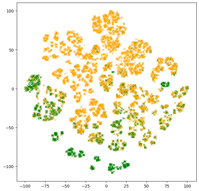
觀察結果

• 存在顏色相似的點叢集。這些範例很容易讓模型分類。
• 存在多個顏色相同的叢集。這些多個叢集顯示具有相同標籤的範例，但根據模型，「原因不同」。
• 顏色混合的叢集包含模型效能不佳的範例。在上面的部分中，我們評估了模型的測試準確度約為 86%。這些很可能就是這些範例。

先前的圖像是靜態圖像。讓我們將其轉換為互動式圖表並檢查個別範例。

# docs_infra: no_execute

# Note: Run the colab (click the "Run in Google Colab" link at the top) to see
# the interactive plot.

def interactive_plot(dataset, projections):

  def label_fn(row):
    """HTML printer over each example."""
    return "<br>".join([f"<b>{k}:</b> {v}" for k, v in row.items()])

  labels = list(dataset.apply(label_fn, axis=1).values)
  iplot({
      "data": [
          go.Scatter(
              x=projections[:, 0],
              y=projections[:, 1],
              text=labels,
              mode="markers",
              marker={
                  "color": colors,
                  "size": 3,
              })
      ],
      "layout": go.Layout(width=600, height=600, template="simple_white")
  })


interactive_plot(test_df, t_sne)

說明：將滑鼠指標放在一些範例上，並嘗試理解它們。將它們與鄰居進行比較。

看不到互動式圖表？：使用 此連結 執行 Colab 以查看互動式圖表。

我們可以根據每個特徵值為範例著色，而不是根據標籤值為範例著色

# Number of columns and rows in the multi-plot.
num_plot_cols = 5
num_plot_rows = math.ceil(test_df.shape[1] / num_plot_cols)

# Color palette for the categorical features.
palette = list(mcolors.TABLEAU_COLORS.values())

# Create the plot
plot_size_in = 3.5
fig, axs = plt.subplots(
    num_plot_rows,
    num_plot_cols,
    figsize=(num_plot_cols * plot_size_in, num_plot_rows * plot_size_in))

# Hide the borders.
for row in axs:
  for ax in row:
    ax.set_axis_off()

for col_idx, col_name in enumerate(test_df):
  ax = axs[col_idx // num_plot_cols, col_idx % num_plot_cols]

  colors = test_df[col_name]
  if colors.dtypes in [str, object]:
    # Use the color palette on categorical features.
    unique_values = list(colors.unique())
    colors = colors.map(
        lambda x: palette[unique_values.index(x) % len(palette)])

  ax.set_title(col_name)
  ax.scatter(t_sne[:, 0], t_sne[:, 1], c=colors.values, linewidths=0.5,
      marker="x", s=5)

原型

透過查看範例的所有鄰居來理解範例並不總是有效率的。相反地，我們可以「群組」相似的範例以簡化此任務。這是原型背後的潛在概念。

原型是範例，不一定在原始資料集中，而是代表資料集中的大型趨勢。查看原型是理解資料集的解決方案。如需更多詳細資訊，請參閱 Molnar 的 Interpretable Machine Learning 的 第 8.7 章。

可以使用不同的方式計算原型，例如使用分群演算法。相反地，Breiman 提出基於簡單迭代演算法的特定解決方案。演算法如下

1. 在 k 個最近鄰居中，選取被最多相同類別的鄰居包圍的範例。
2. 使用選取範例及其 k 個鄰居的中位數特徵值建立原型範例。
3. 移除這 k+1 個範例
4. 重複

非正式地說，原型是我們上面建立的圖表中叢集的中心。

讓我們實作此演算法並查看一些原型。

首先是選取步驟 1 中範例的方法。

def select_example(labels, distance_matrix, k):
  """Selects the example with the highest number of neighbors with the same class.

  Usage example:
    n = 5
    select_example(
        np.random.randint(0,2, size=n),
        np.random.uniform(size=(n,n)),
        2)

  Returns:
    The list of neighbors for the selected example. Includes the selected
    example.
  """

  partition = np.argpartition(distance_matrix, k)[:,:k]
  same_label = np.mean(np.equal(labels[partition], np.expand_dims(labels, axis=1)), axis=1)
  selected_example = np.argmax(same_label)
  return partition[selected_example, :]

def extract_prototype_examples(labels, distance_matrix, k, num_prototypes):
  """Extracts a list of examples in each prototype.

  Usage example:
    n = 50
    print(extract_prototype_examples(
        labels=np.random.randint(0, 2, size=n),
        distance_matrix=np.random.uniform(size=(n, n)),
        k=2,
        num_prototypes=3))

  Returns:
    An array where E[i][j] is the index of the j-th examples of the i-th
    prototype. 
  """

  example_idxs = np.arange(len(labels))
  prototypes = []
  examples_per_prototype = []

  for iter in range(num_prototypes):
    print(f"Iter #{iter}")
    # Select the example
    neighbors = select_example(labels, distance_matrix, k)

    # Index of the examples in the prototype
    examples_per_prototype.append(list(example_idxs[neighbors]))

    # Remove the selected examples
    example_idxs = np.delete(example_idxs, neighbors)
    labels = np.delete(labels, neighbors)
    distance_matrix = np.delete(distance_matrix, neighbors, axis=0)
    distance_matrix = np.delete(distance_matrix, neighbors, axis=1)

  return examples_per_prototype

使用上述方法，讓我們擷取 10 個原型的範例。

examples_per_prototype = extract_prototype_examples(test_df["income"].values, distance, k=20, num_prototypes=10)
print(f"Found examples for {len(examples_per_prototype)} prototypes.")

Iter #0
Iter #1
Iter #2
Iter #3
Iter #4
Iter #5
Iter #6
Iter #7
Iter #8
Iter #9
Found examples for 10 prototypes.

對於每個原型，我們想要顯示特徵值的統計資訊。在此範例中，我們將查看數值特徵的四分位數，以及類別特徵的最頻繁值。

def build_prototype(dataset):
  """Exacts the feature statistics of a prototype.

  For numerical features, returns the quantiles.
  For categorical features, returns the most frequent value.

  Usage example:
    n = 50
    print(build_prototype(
        pd.DataFrame({
            "f1": np.random.uniform(size=n),
            "f2": np.random.uniform(size=n),
            "f3": [f"v_{x}" for x in np.random.randint(0, 2, size=n)],
            "label": np.random.randint(0, 2, size=n)
        })))

  Return:
    A prototype as a dictionary of strings.
  """

  prototype = {}
  for col in dataset.columns:
    col_values = dataset[col]
    if col_values.dtypes in [str, object]:
      # A categorical feature.

      # Remove the missing values
      col_values = [x for x in col_values if isinstance(x,str) or not math.isnan(x)]

      # Frequency of each possible value.
      frequency_item, frequency_count = np.unique(col_values, return_counts=True)
      top_item_idx = np.argmax(frequency_count)
      top_item_probability = frequency_count[top_item_idx] / np.sum(frequency_count)

      # Print the most common item.
      prototype[col] = f"{frequency_item[top_item_idx]} ({100*top_item_probability:.0f}%)"

    else:
      # A numerical feature.
      quartiles = np.nanquantile(col_values.values, [0.25, 0.5, 0.75])
      # Print the 3 quantiles.
      prototype[col] = f"{quartiles[0]} {quartiles[1]} {quartiles[2]}"
  return prototype

現在，讓我們看看我們的原型。

# Extract the statistics of each prototype.
prototypes = []
for examples in examples_per_prototype:
  # Prorotype statistics.
  prototypes.append(build_prototype(test_df.iloc[examples, :]))
prototypes = pd.DataFrame(prototypes)

prototypes

嘗試理解原型。

讓我們擷取並繪製這些原型中元素平均 2d t-SNE 投影。

# Extract the projection of each prototype.
prototypes_projection = []
for examples in examples_per_prototype:
  # t-SNE for each prototype.
  prototypes_projection.append(np.mean(t_sne[examples,:],axis=0))
prototypes_projection = np.stack(prototypes_projection)

# Plot the mean 2d t-SNE projection of the elements in the prototypes.

fig, ax = plt.subplots(1, 1, figsize=(8, 8))
ax.grid(False)

# Color the points according to the label value.
colors = (test_df["income"] == ">50K").map(lambda x: ["orange", "green"][x])
ax.scatter(
    t_sne[:, 0], t_sne[:, 1], c=colors, linewidths=0.5, marker="x", s=20)

# Add the prototype indices.
for i in range(prototypes_projection.shape[0]):
  ax.text(prototypes_projection[i, 0],
          prototypes_projection[i, 1],
          f"{i}",
          fontdict={"size":18},
          c="red")

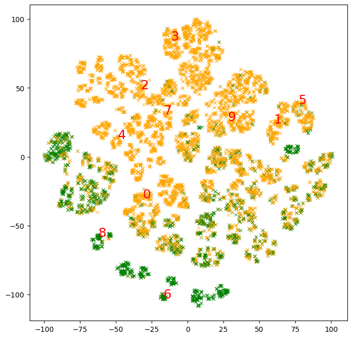
我們看到 10 個原型涵蓋了大約一半的領域。沒有原型的範例叢集最好用更多原型來解釋。

在上面的範例中，我們自動擷取了原型。但是，我們也可以圍繞特定範例建立原型。

讓我們圍繞範例 #0 建立原型。

example_idx = 0
k = 20
neighbors = np.argpartition(distance[example_idx, :], k)[:k]

print(f"The example #{example_idx} is:")
print("===============================")
print(test_df.iloc[example_idx, :])
print("")
print(f"The prototype around the example #{example_idx} is:")
print("============================================")
print(pd.Series(build_prototype(test_df.iloc[neighbors, :])))

The example #0 is:
===============================
age                          39
workclass             State-gov
fnlwgt                    77516
education             Bachelors
education_num                13
marital_status    Never-married
occupation         Adm-clerical
relationship      Not-in-family
race                      White
sex                        Male
capital_gain               2174
capital_loss                  0
hours_per_week               40
native_country    United-States
income                    <=50K
Name: 0, dtype: object

The prototype around the example #0 is:
============================================
age                          36.0 39.0 41.0
workclass                     Private (50%)
fnlwgt            72314.0 115188.5 138797.0
education                   Bachelors (95%)
education_num                13.0 13.0 13.0
marital_status          Never-married (65%)
occupation               Adm-clerical (70%)
relationship            Not-in-family (75%)
race                            White (95%)
sex                              Male (65%)
capital_gain                    0.0 0.0 0.0
capital_loss                    0.0 0.0 0.0
hours_per_week              38.75 40.0 40.0
native_country         United-States (100%)
income                         <=50K (100%)
dtype: object