
|
|
|
 在 GitHub 上檢視 在 GitHub 上檢視
|
|
|
簡介
歡迎使用 TensorFlow Decision Forests (TF-DF) 的模型組合教學課程。這個筆記本向您展示如何使用常見的預先處理層和 Keras Functional API,將多個決策樹森林和神經網路模型組合在一起。
您可能會想要將模型組合在一起,以改善預測效能 (集成學習)、充分利用不同建模技術的優勢 (異質模型集成)、在不同資料集上訓練模型的不同部分 (例如預先訓練),或建立堆疊模型 (例如,一個模型對另一個模型的預測進行操作)。
本教學課程涵蓋使用 Functional API 的模型組合進階使用案例。您可以在這個教學課程的「特徵預先處理」章節和這個教學課程的「使用預先訓練的文字嵌入」章節中找到更簡單的模型組合情境範例。
以下是您將建構的模型結構

您的組合模型有三個階段
- 第一階段是預先處理層,由神經網路組成,且為下一階段中的所有模型通用。實際上,這樣的預先處理層可以是微調的預先訓練嵌入,也可以是隨機初始化的神經網路。
- 第二階段是兩個決策樹森林和兩個神經網路模型的集成。
- 最後階段是平均第二階段中模型的預測。它不包含任何可學習的權重。
神經網路使用反向傳播演算法和梯度下降法進行訓練。此演算法具有兩個重要屬性:(1) 如果神經網路層接收到損失梯度 (更精確地說,是損失根據層輸出的梯度),則可以訓練該層神經網路,以及 (2) 演算法將損失梯度從層的輸出「傳輸」到層的輸入 (這是「鏈式法則」)。基於這兩個原因,反向傳播可以一起訓練堆疊在彼此之上的多個神經網路層。
在這個範例中,決策樹森林使用隨機森林 (RF) 演算法進行訓練。與反向傳播不同,RF 的訓練不會將損失梯度從其輸出「傳輸」到其輸入。基於這些原因,傳統的 RF 演算法不能用於訓練或微調底層的神經網路。換句話說,「決策樹森林」階段不能用於訓練「可學習的 NN 預先處理區塊」。
- 訓練預先處理和神經網路階段。
- 訓練決策樹森林階段。
安裝 TensorFlow Decision Forests
執行以下儲存格以安裝 TF-DF。
pip install tensorflow_decision_forests -U --quiet
需要 Wurlitzer 才能在 Colabs 中顯示詳細的訓練記錄 (當在模型建構函式中使用 verbose=2 時)。
pip install wurlitzer -U --quiet
匯入程式庫
import os
# Keep using Keras 2
os.environ['TF_USE_LEGACY_KERAS'] = '1'

import tensorflow_decision_forests as tfdf

import numpy as np
import pandas as pd
import tensorflow as tf
import tf_keras
import math
import matplotlib.pyplot as plt
資料集
在本教學課程中,您將使用簡單的合成資料集,以便更輕鬆地解讀最終模型。
def make_dataset(num_examples, num_features, seed=1234):
  np.random.seed(seed)
  features = np.random.uniform(-1, 1, size=(num_examples, num_features))
  noise = np.random.uniform(size=(num_examples))

  left_side = np.sqrt(
      np.sum(np.multiply(np.square(features[:, 0:2]), [1, 2]), axis=1))
  right_side = features[:, 2] * 0.7 + np.sin(
      features[:, 3] * 10) * 0.5 + noise * 0.0 + 0.5

  labels = left_side <= right_side
  return features, labels.astype(int)
產生一些範例
make_dataset(num_examples=5, num_features=4)
(array([[-0.6169611 ,  0.24421754, -0.12454452,  0.57071717],
        [ 0.55995162, -0.45481479, -0.44707149,  0.60374436],
        [ 0.91627871,  0.75186527, -0.28436546,  0.00199025],
        [ 0.36692587,  0.42540405, -0.25949849,  0.12239237],
        [ 0.00616633, -0.9724631 ,  0.54565324,  0.76528238]]),
 array([0, 0, 0, 1, 0]))
您也可以繪製這些範例,以瞭解合成模式
plot_features, plot_label = make_dataset(num_examples=50000, num_features=4)

plt.rcParams["figure.figsize"] = [8, 8]
common_args = dict(c=plot_label, s=1.0, alpha=0.5)

plt.subplot(2, 2, 1)
plt.scatter(plot_features[:, 0], plot_features[:, 1], **common_args)

plt.subplot(2, 2, 2)
plt.scatter(plot_features[:, 1], plot_features[:, 2], **common_args)

plt.subplot(2, 2, 3)
plt.scatter(plot_features[:, 0], plot_features[:, 2], **common_args)

plt.subplot(2, 2, 4)
plt.scatter(plot_features[:, 0], plot_features[:, 3], **common_args)
<matplotlib.collections.PathCollection at 0x7f4a523ddca0>
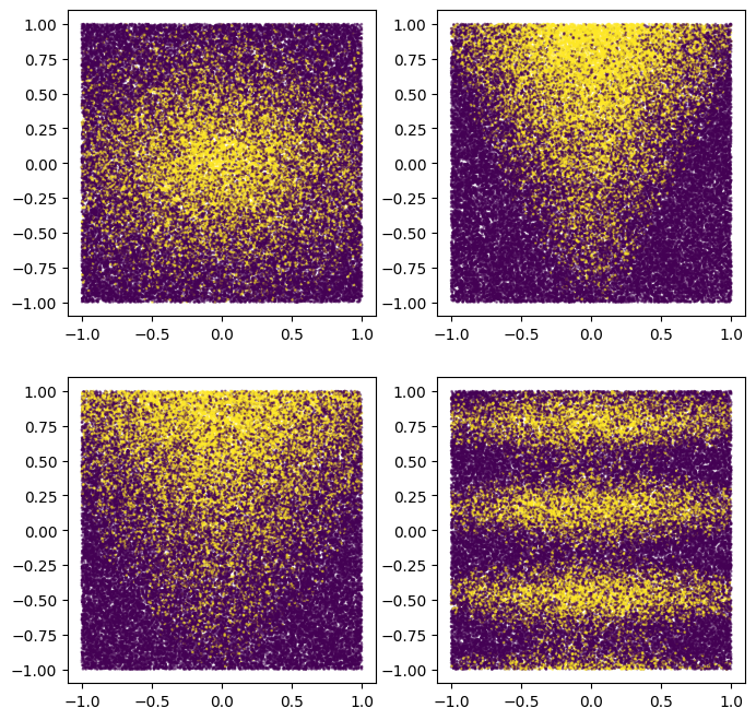
請注意,此模式是平滑且未與軸對齊的。這將有利於神經網路模型。這是因為對於神經網路而言,比決策樹更容易具有圓形和非對齊的決策邊界。
另一方面,我們將在包含 2500 個範例的小型資料集上訓練模型。這將有利於決策樹森林模型。這是因為決策樹森林效率更高,可以利用範例中的所有可用資訊 (決策樹森林是「樣本有效率的」)。
我們的神經網路和決策樹森林集成將充分利用兩者的優勢。
讓我們建立訓練和測試 tf.data.Dataset
def make_tf_dataset(batch_size=64, **args):
  features, labels = make_dataset(**args)
  return tf.data.Dataset.from_tensor_slices(
      (features, labels)).batch(batch_size)


num_features = 10

train_dataset = make_tf_dataset(
    num_examples=2500, num_features=num_features, batch_size=100, seed=1234)
test_dataset = make_tf_dataset(
    num_examples=10000, num_features=num_features, batch_size=100, seed=5678)
模型結構
如下定義模型結構
# Input features.
raw_features = tf_keras.layers.Input(shape=(num_features,))

# Stage 1
# =======

# Common learnable pre-processing
preprocessor = tf_keras.layers.Dense(10, activation=tf.nn.relu6)
preprocess_features = preprocessor(raw_features)

# Stage 2
# =======

# Model #1: NN
m1_z1 = tf_keras.layers.Dense(5, activation=tf.nn.relu6)(preprocess_features)
m1_pred = tf_keras.layers.Dense(1, activation=tf.nn.sigmoid)(m1_z1)

# Model #2: NN
m2_z1 = tf_keras.layers.Dense(5, activation=tf.nn.relu6)(preprocess_features)
m2_pred = tf_keras.layers.Dense(1, activation=tf.nn.sigmoid)(m2_z1)


# Model #3: DF
model_3 = tfdf.keras.RandomForestModel(num_trees=1000, random_seed=1234)
m3_pred = model_3(preprocess_features)

# Model #4: DF
model_4 = tfdf.keras.RandomForestModel(
    num_trees=1000,
    #split_axis="SPARSE_OBLIQUE", # Uncomment this line to increase the quality of this model
    random_seed=4567)
m4_pred = model_4(preprocess_features)

# Since TF-DF uses deterministic learning algorithms, you should set the model's
# training seed to different values otherwise both
# `tfdf.keras.RandomForestModel` will be exactly the same.

# Stage 3
# =======

mean_nn_only = tf.reduce_mean(tf.stack([m1_pred, m2_pred], axis=0), axis=0)
mean_nn_and_df = tf.reduce_mean(
    tf.stack([m1_pred, m2_pred, m3_pred, m4_pred], axis=0), axis=0)

# Keras Models
# ============

ensemble_nn_only = tf_keras.models.Model(raw_features, mean_nn_only)
ensemble_nn_and_df = tf_keras.models.Model(raw_features, mean_nn_and_df)
Warning: The `num_threads` constructor argument is not set and the number of CPU is os.cpu_count()=32 > 32. Setting num_threads to 32. Set num_threads manually to use more than 32 cpus.
WARNING:absl:The `num_threads` constructor argument is not set and the number of CPU is os.cpu_count()=32 > 32. Setting num_threads to 32. Set num_threads manually to use more than 32 cpus.
Use /tmpfs/tmp/tmp5rudwfpk as temporary training directory
Warning: The model was called directly (i.e. using `model(data)` instead of using `model.predict(data)`) before being trained. The model will only return zeros until trained. The output shape might change after training Tensor("inputs:0", shape=(None, 10), dtype=float32)
WARNING:absl:The model was called directly (i.e. using `model(data)` instead of using `model.predict(data)`) before being trained. The model will only return zeros until trained. The output shape might change after training Tensor("inputs:0", shape=(None, 10), dtype=float32)
Warning: The `num_threads` constructor argument is not set and the number of CPU is os.cpu_count()=32 > 32. Setting num_threads to 32. Set num_threads manually to use more than 32 cpus.
WARNING:absl:The `num_threads` constructor argument is not set and the number of CPU is os.cpu_count()=32 > 32. Setting num_threads to 32. Set num_threads manually to use more than 32 cpus.
Use /tmpfs/tmp/tmp7z3k5oog as temporary training directory
Warning: The model was called directly (i.e. using `model(data)` instead of using `model.predict(data)`) before being trained. The model will only return zeros until trained. The output shape might change after training Tensor("inputs:0", shape=(None, 10), dtype=float32)
WARNING:absl:The model was called directly (i.e. using `model(data)` instead of using `model.predict(data)`) before being trained. The model will only return zeros until trained. The output shape might change after training Tensor("inputs:0", shape=(None, 10), dtype=float32)
在訓練模型之前,您可以繪製模型以檢查它是否與初始圖表相似。
from keras.utils import plot_model

plot_model(ensemble_nn_and_df, to_file="/tmp/model.png", show_shapes=True)
模型訓練
首先使用反向傳播演算法訓練預先處理和兩個神經網路層。
%%time
ensemble_nn_only.compile(
        optimizer=tf_keras.optimizers.Adam(),
        loss=tf_keras.losses.BinaryCrossentropy(),
        metrics=["accuracy"])

ensemble_nn_only.fit(train_dataset, epochs=20, validation_data=test_dataset)
Epoch 1/20
WARNING: All log messages before absl::InitializeLog() is called are written to STDERR
I0000 00:00:1713611529.601020   11701 service.cc:145] XLA service 0x7f48904d48d0 initialized for platform CUDA (this does not guarantee that XLA will be used). Devices:
I0000 00:00:1713611529.601060   11701 service.cc:153]   StreamExecutor device (0): Tesla T4, Compute Capability 7.5
I0000 00:00:1713611529.601064   11701 service.cc:153]   StreamExecutor device (1): Tesla T4, Compute Capability 7.5
I0000 00:00:1713611529.601067   11701 service.cc:153]   StreamExecutor device (2): Tesla T4, Compute Capability 7.5
I0000 00:00:1713611529.601069   11701 service.cc:153]   StreamExecutor device (3): Tesla T4, Compute Capability 7.5
I0000 00:00:1713611529.771938   11701 device_compiler.h:188] Compiled cluster using XLA!  This line is logged at most once for the lifetime of the process.
25/25 [==============================] - 15s 33ms/step - loss: 0.5756 - accuracy: 0.7500 - val_loss: 0.5714 - val_accuracy: 0.7392
Epoch 2/20
25/25 [==============================] - 0s 11ms/step - loss: 0.5524 - accuracy: 0.7500 - val_loss: 0.5543 - val_accuracy: 0.7392
Epoch 3/20
25/25 [==============================] - 0s 10ms/step - loss: 0.5351 - accuracy: 0.7500 - val_loss: 0.5406 - val_accuracy: 0.7392
Epoch 4/20
25/25 [==============================] - 0s 10ms/step - loss: 0.5209 - accuracy: 0.7500 - val_loss: 0.5287 - val_accuracy: 0.7392
Epoch 5/20
25/25 [==============================] - 0s 10ms/step - loss: 0.5083 - accuracy: 0.7500 - val_loss: 0.5176 - val_accuracy: 0.7392
Epoch 6/20
25/25 [==============================] - 0s 10ms/step - loss: 0.4967 - accuracy: 0.7500 - val_loss: 0.5072 - val_accuracy: 0.7392
Epoch 7/20
25/25 [==============================] - 0s 10ms/step - loss: 0.4856 - accuracy: 0.7512 - val_loss: 0.4973 - val_accuracy: 0.7397
Epoch 8/20
25/25 [==============================] - 0s 10ms/step - loss: 0.4753 - accuracy: 0.7524 - val_loss: 0.4882 - val_accuracy: 0.7421
Epoch 9/20
25/25 [==============================] - 0s 10ms/step - loss: 0.4658 - accuracy: 0.7572 - val_loss: 0.4799 - val_accuracy: 0.7454
Epoch 10/20
25/25 [==============================] - 0s 10ms/step - loss: 0.4572 - accuracy: 0.7600 - val_loss: 0.4726 - val_accuracy: 0.7500
Epoch 11/20
25/25 [==============================] - 0s 10ms/step - loss: 0.4498 - accuracy: 0.7668 - val_loss: 0.4664 - val_accuracy: 0.7575
Epoch 12/20
25/25 [==============================] - 0s 10ms/step - loss: 0.4435 - accuracy: 0.7748 - val_loss: 0.4612 - val_accuracy: 0.7637
Epoch 13/20
25/25 [==============================] - 0s 11ms/step - loss: 0.4382 - accuracy: 0.7780 - val_loss: 0.4569 - val_accuracy: 0.7678
Epoch 14/20
25/25 [==============================] - 0s 10ms/step - loss: 0.4339 - accuracy: 0.7832 - val_loss: 0.4534 - val_accuracy: 0.7702
Epoch 15/20
25/25 [==============================] - 0s 11ms/step - loss: 0.4302 - accuracy: 0.7888 - val_loss: 0.4504 - val_accuracy: 0.7731
Epoch 16/20
25/25 [==============================] - 0s 10ms/step - loss: 0.4269 - accuracy: 0.7920 - val_loss: 0.4477 - val_accuracy: 0.7768
Epoch 17/20
25/25 [==============================] - 0s 10ms/step - loss: 0.4239 - accuracy: 0.7924 - val_loss: 0.4452 - val_accuracy: 0.7786
Epoch 18/20
25/25 [==============================] - 0s 10ms/step - loss: 0.4211 - accuracy: 0.7936 - val_loss: 0.4429 - val_accuracy: 0.7800
Epoch 19/20
25/25 [==============================] - 0s 10ms/step - loss: 0.4184 - accuracy: 0.7976 - val_loss: 0.4406 - val_accuracy: 0.7819
Epoch 20/20
25/25 [==============================] - 0s 10ms/step - loss: 0.4158 - accuracy: 0.7992 - val_loss: 0.4382 - val_accuracy: 0.7836
CPU times: user 20.7 s, sys: 1.36 s, total: 22 s
Wall time: 19.6 s
<tf_keras.src.callbacks.History at 0x7f4a4c0fa3a0>
讓我們評估預先處理和僅包含兩個神經網路的部分
evaluation_nn_only = ensemble_nn_only.evaluate(test_dataset, return_dict=True)
print("Accuracy (NN #1 and #2 only): ", evaluation_nn_only["accuracy"])
print("Loss (NN #1 and #2 only): ", evaluation_nn_only["loss"])
100/100 [==============================] - 0s 2ms/step - loss: 0.4382 - accuracy: 0.7836
Accuracy (NN #1 and #2 only):  0.7835999727249146
Loss (NN #1 and #2 only):  0.438231498003006
讓我們 (依序) 訓練兩個決策樹森林元件。
%%time
train_dataset_with_preprocessing = train_dataset.map(lambda x,y: (preprocessor(x), y))
test_dataset_with_preprocessing = test_dataset.map(lambda x,y: (preprocessor(x), y))

model_3.fit(train_dataset_with_preprocessing)
model_4.fit(train_dataset_with_preprocessing)
WARNING:tensorflow:AutoGraph could not transform <function <lambda> at 0x7f4b7b5d91f0> and will run it as-is.
Cause: could not parse the source code of <function <lambda> at 0x7f4b7b5d91f0>: no matching AST found among candidates:

To silence this warning, decorate the function with @tf.autograph.experimental.do_not_convert
WARNING: AutoGraph could not transform <function <lambda> at 0x7f4b7b5d91f0> and will run it as-is.
Cause: could not parse the source code of <function <lambda> at 0x7f4b7b5d91f0>: no matching AST found among candidates:

To silence this warning, decorate the function with @tf.autograph.experimental.do_not_convert
WARNING:tensorflow:AutoGraph could not transform <function <lambda> at 0x7f4b7ba3eee0> and will run it as-is.
Cause: could not parse the source code of <function <lambda> at 0x7f4b7ba3eee0>: no matching AST found among candidates:

To silence this warning, decorate the function with @tf.autograph.experimental.do_not_convert
WARNING: AutoGraph could not transform <function <lambda> at 0x7f4b7ba3eee0> and will run it as-is.
Cause: could not parse the source code of <function <lambda> at 0x7f4b7ba3eee0>: no matching AST found among candidates:

To silence this warning, decorate the function with @tf.autograph.experimental.do_not_convert
Reading training dataset...
Training dataset read in 0:00:03.699343. Found 2500 examples.
Training model...
[INFO 24-04-20 11:12:20.9165 UTC kernel.cc:1233] Loading model from path /tmpfs/tmp/tmp5rudwfpk/model/ with prefix 3da3a8649d9e4cb4
Model trained in 0:00:02.061496
Compiling model...
[INFO 24-04-20 11:12:22.0091 UTC decision_forest.cc:734] Model loaded with 1000 root(s), 355690 node(s), and 10 input feature(s).
[INFO 24-04-20 11:12:22.0091 UTC abstract_model.cc:1344] Engine "RandomForestOptPred" built
[INFO 24-04-20 11:12:22.0091 UTC kernel.cc:1061] Use fast generic engine
Model compiled.
Reading training dataset...
Training dataset read in 0:00:00.231041. Found 2500 examples.
Training model...
[INFO 24-04-20 11:12:23.7301 UTC kernel.cc:1233] Loading model from path /tmpfs/tmp/tmp7z3k5oog/model/ with prefix 8b0da5e131c043b2
Model trained in 0:00:01.916593
Compiling model...
[INFO 24-04-20 11:12:24.7575 UTC decision_forest.cc:734] Model loaded with 1000 root(s), 357028 node(s), and 10 input feature(s).
[INFO 24-04-20 11:12:24.7576 UTC kernel.cc:1061] Use fast generic engine
Model compiled.
CPU times: user 22.9 s, sys: 1.73 s, total: 24.6 s
Wall time: 8.74 s
<tf_keras.src.callbacks.History at 0x7f4b7b6fcee0>
讓我們個別評估決策樹森林。
model_3.compile(["accuracy"])
model_4.compile(["accuracy"])

evaluation_df3_only = model_3.evaluate(
    test_dataset_with_preprocessing, return_dict=True)
evaluation_df4_only = model_4.evaluate(
    test_dataset_with_preprocessing, return_dict=True)

print("Accuracy (DF #3 only): ", evaluation_df3_only["accuracy"])
print("Accuracy (DF #4 only): ", evaluation_df4_only["accuracy"])
100/100 [==============================] - 2s 10ms/step - loss: 0.0000e+00 - accuracy: 0.7990
100/100 [==============================] - 1s 10ms/step - loss: 0.0000e+00 - accuracy: 0.7989
Accuracy (DF #3 only):  0.7990000247955322
Accuracy (DF #4 only):  0.7989000082015991
讓我們評估整個模型組合
ensemble_nn_and_df.compile(
    loss=tf_keras.losses.BinaryCrossentropy(), metrics=["accuracy"])

evaluation_nn_and_df = ensemble_nn_and_df.evaluate(
    test_dataset, return_dict=True)

print("Accuracy (2xNN and 2xDF): ", evaluation_nn_and_df["accuracy"])
print("Loss (2xNN and 2xDF): ", evaluation_nn_and_df["loss"])
100/100 [==============================] - 2s 10ms/step - loss: 0.4226 - accuracy: 0.7953
Accuracy (2xNN and 2xDF):  0.7953000068664551
Loss (2xNN and 2xDF):  0.4225609302520752
最後,讓我們稍微微調神經網路層。請注意,我們不會微調預先訓練的嵌入,因為 DF 模型依賴它 (除非我們也會在之後重新訓練它們)。
總而言之,您有
Accuracy (NN #1 and #2 only): 0.783600
Accuracy (DF #3 only):        0.799000
Accuracy (DF #4 only):        0.798900
----------------------------------------
Accuracy (2xNN and 2xDF): 0.795300
                  +0.011700 over NN #1 and #2 only
                  -0.003700 over DF #3 only
                  -0.003600 over DF #4 only
在這裡,您可以看到組合模型的效能優於其個別部分。這就是集成學習如此有效的原因。
下一步?
在這個範例中,您瞭解了如何將決策樹森林與神經網路結合。額外的步驟是進一步一起訓練神經網路和決策樹森林。
此外,為了清楚起見,決策樹森林僅接收預先處理的輸入。但是,決策樹森林通常非常適合使用原始資料。透過也將原始特徵饋送到決策樹森林模型,可以改進模型。
在這個範例中,最終模型是個別模型預測的平均值。如果所有模型的效能大致相同,則此解決方案效果良好。但是,如果其中一個子模型非常好,則將其與其他模型聚合實際上可能有害 (反之亦然;例如,嘗試將範例數量從 1k 減少,看看它對神經網路的影響有多大;或在第二個隨機森林模型中啟用 SPARSE_OBLIQUE 分裂)。