使用 Transformer 和 Keras 進行神經機器翻譯

在 TensorFlow.org 上檢視

在 Google Colab 中執行

在 GitHub 上檢視原始碼

下載筆記本

本教學課程示範如何建立及訓練 序列到序列 Transformer 模型，以將 葡萄牙文翻譯成英文。Transformer 最初由 Vaswani 等人在 「Attention is all you need」(注意力機制就是你所需要的一切) (2017) 中提出。

Transformer 是深度神經網路，以自我注意力機制取代 CNN 和 RNN。自我注意力機制讓 Transformer 能夠輕鬆地在輸入序列之間傳輸資訊。

如 Google AI 部落格文章中所述

用於機器翻譯的神經網路通常包含一個編碼器，用於讀取輸入句子並產生其表示法。然後，解碼器會逐字產生輸出句子，同時參考編碼器產生的表示法。Transformer 首先為每個字詞產生初始表示法或嵌入。然後，透過使用自我注意力機制，它會彙總來自所有其他字詞的資訊，為每個字詞產生由整個脈絡 (以填滿的球體表示) 通知的新表示法。接著，會針對所有字詞平行重複此步驟多次，依序產生新的表示法。

圖 1：將 Transformer 應用於機器翻譯。來源：Google AI 部落格。

這需要消化大量資訊，本教學課程的目標是將其分解為易於理解的部分。在本教學課程中，您將

• 準備資料。
• 實作必要元件
  • 位置嵌入。
  • 注意力層。
  • 編碼器和解碼器。
• 建構及訓練 Transformer。
• 產生翻譯。
• 匯出模型。

為了充分利用本教學課程，如果您了解文字產生的基本概念和注意力機制，將會有所幫助。

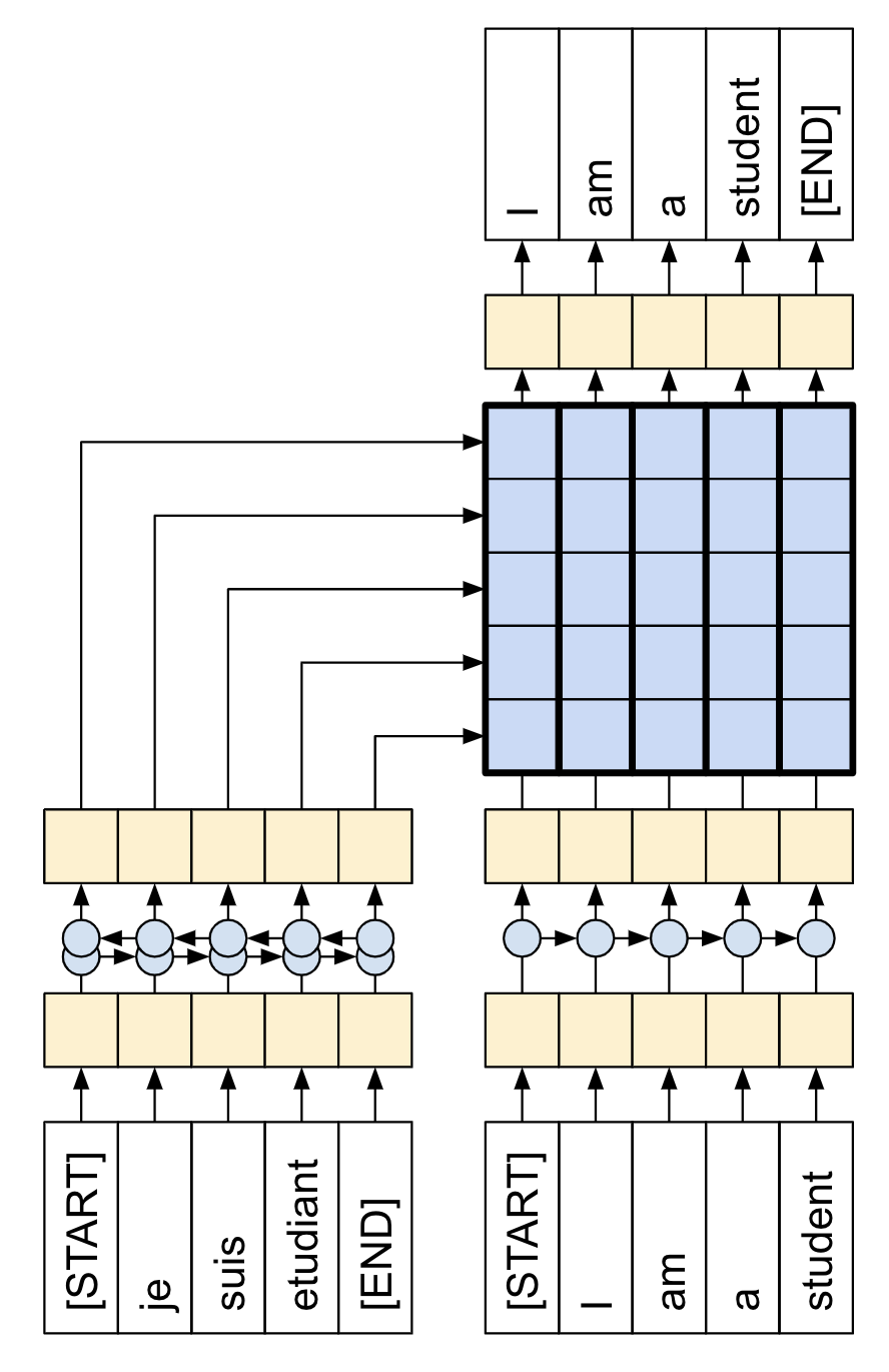
Transformer 是一種序列到序列編碼器-解碼器模型，類似於使用注意力機制的 NMT 教學課程中的模型。單層 Transformer 需要編寫更多程式碼，但幾乎與該編碼器-解碼器 RNN 模型相同。唯一的區別在於 RNN 層被自我注意力層取代。本教學課程建構了一個 4 層 Transformer，它更大且更強大，但從根本上來說並非更複雜。

RNN+注意力機制模型	單層 Transformer

在本筆記本中訓練模型後，您將能夠輸入葡萄牙文句子並傳回英文翻譯。

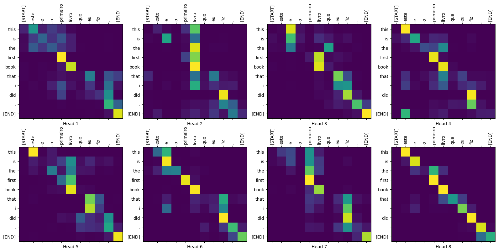
圖 2：在本教學課程結束時您可以產生的視覺化注意力權重。

Transformer 為何如此重要

• Transformer 擅長對循序資料 (例如自然語言) 進行建模。
• 與 循環神經網路 (RNN) 不同，Transformer 是可平行化的。這使它們在 GPU 和 TPU 等硬體上更有效率。主要原因是 Transformer 以注意力機制取代了循環，而且計算可以同時進行。層輸出可以平行計算，而不是像 RNN 那樣的序列。
• 與 RNN (例如 seq2seq, 2014) 或 卷積神經網路 (CNN) (例如 ByteNet) 不同，Transformer 能夠擷取資料中遠距離或長距離脈絡和依賴關係，介於輸入或輸出序列中的遠距離位置之間。因此，可以學習更長的連線。注意力機制允許每個位置在每一層存取整個輸入，而在 RNN 和 CNN 中，資訊需要通過許多處理步驟才能移動長距離，這使得學習更加困難。
• Transformer 對資料的時序/空間關係不做假設。這非常適合處理一組物件 (例如，星海爭霸單位)。

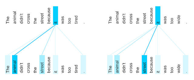
圖 3：針對英法翻譯訓練的 Transformer 的第 5 層到第 6 層中，字詞「it」的編碼器自我注意力分佈 (八個注意力頭之一)。來源：Google AI 部落格。

設定

首先安裝 TensorFlow Datasets 以載入資料集，並安裝 TensorFlow Text 以進行文字預處理

# Install the most re version of TensorFlow to use the improved
# masking support for `tf.keras.layers.MultiHeadAttention`.
apt install --allow-change-held-packages libcudnn8=8.1.0.77-1+cuda11.2
pip uninstall -y -q tensorflow keras tensorflow-estimator tensorflow-text
pip install protobuf~=3.20.3
pip install -q tensorflow_datasets
pip install -q -U tensorflow-text tensorflow

匯入必要的模組

import logging
import time

import numpy as np
import matplotlib.pyplot as plt

import tensorflow_datasets as tfds
import tensorflow as tf

import tensorflow_text

資料處理

本節從 本教學課程下載資料集和子詞權杖產生器，然後將它們全部封裝在 tf.data.Dataset 中以進行訓練。

examples, metadata = tfds.load('ted_hrlr_translate/pt_to_en',
                               with_info=True,
                               as_supervised=True)

train_examples, val_examples = examples['train'], examples['validation']

for pt_examples, en_examples in train_examples.batch(3).take(1):
  print('> Examples in Portuguese:')
  for pt in pt_examples.numpy():
    print(pt.decode('utf-8'))
  print()

  print('> Examples in English:')
  for en in en_examples.numpy():
    print(en.decode('utf-8'))

model_name = 'ted_hrlr_translate_pt_en_converter'
tf.keras.utils.get_file(
    f'{model_name}.zip',
    f'https://storage.googleapis.com/download.tensorflow.org/models/{model_name}.zip',
    cache_dir='.', cache_subdir='', extract=True
)

tokenizers = tf.saved_model.load(model_name)

[item for item in dir(tokenizers.en) if not item.startswith('_')]

print('> This is a batch of strings:')
for en in en_examples.numpy():
  print(en.decode('utf-8'))

encoded = tokenizers.en.tokenize(en_examples)

print('> This is a padded-batch of token IDs:')
for row in encoded.to_list():
  print(row)

round_trip = tokenizers.en.detokenize(encoded)

print('> This is human-readable text:')
for line in round_trip.numpy():
  print(line.decode('utf-8'))

print('> This is the text split into tokens:')
tokens = tokenizers.en.lookup(encoded)
tokens

lengths = []

for pt_examples, en_examples in train_examples.batch(1024):
  pt_tokens = tokenizers.pt.tokenize(pt_examples)
  lengths.append(pt_tokens.row_lengths())

  en_tokens = tokenizers.en.tokenize(en_examples)
  lengths.append(en_tokens.row_lengths())
  print('.', end='', flush=True)

all_lengths = np.concatenate(lengths)

plt.hist(all_lengths, np.linspace(0, 500, 101))
plt.ylim(plt.ylim())
max_length = max(all_lengths)
plt.plot([max_length, max_length], plt.ylim())
plt.title(f'Maximum tokens per example: {max_length}');

MAX_TOKENS=128
def prepare_batch(pt, en):
    pt = tokenizers.pt.tokenize(pt)      # Output is ragged.
    pt = pt[:, :MAX_TOKENS]    # Trim to MAX_TOKENS.
    pt = pt.to_tensor()  # Convert to 0-padded dense Tensor

    en = tokenizers.en.tokenize(en)
    en = en[:, :(MAX_TOKENS+1)]
    en_inputs = en[:, :-1].to_tensor()  # Drop the [END] tokens
    en_labels = en[:, 1:].to_tensor()   # Drop the [START] tokens

    return (pt, en_inputs), en_labels

BUFFER_SIZE = 20000
BATCH_SIZE = 64

def make_batches(ds):
  return (
      ds
      .shuffle(BUFFER_SIZE)
      .batch(BATCH_SIZE)
      .map(prepare_batch, tf.data.AUTOTUNE)
      .prefetch(buffer_size=tf.data.AUTOTUNE))

測試資料集

# Create training and validation set batches.
train_batches = make_batches(train_examples)
val_batches = make_batches(val_examples)

產生的 tf.data.Dataset 物件已設定為使用 Keras 進行訓練。Keras Model.fit 訓練預期會有 (inputs, labels) 組。inputs 是權杖化的葡萄牙文和英文序列組 (pt, en)。labels 是相同的英文序列，但偏移了 1。此偏移是為了讓每個位置的輸入 en 序列中，label 為下一個權杖。

底部是輸入，頂部是標籤。

這與文字產生教學課程相同，只是這裡您有額外的輸入「脈絡」(葡萄牙文序列)，模型以其為「條件」。

此設定稱為「教師強制」，因為無論模型在每個時間步的輸出為何，它都會取得真實值作為下一個時間步的輸入。這是訓練文字產生模型的一種簡單有效的方法。它之所以有效率，是因為您不需要循序執行模型，不同序列位置的輸出可以平行計算。

您可能預期 input, output 組只是 葡萄牙文、英文 序列。給定葡萄牙文序列，模型會嘗試產生英文序列。

可以透過這種方式訓練模型。您需要寫出推論迴圈，並將模型的輸出傳回輸入。這會比較慢 (時間步無法平行執行)，而且學習任務也更困難 (模型必須先正確取得句子的開頭，才能正確取得結尾)，但它可以提供更穩定的模型，因為模型必須學會在訓練期間更正自己的錯誤。

for (pt, en), en_labels in train_batches.take(1):
  break

print(pt.shape)
print(en.shape)
print(en_labels.shape)

en 和 en_labels 相同，只是偏移了 1

print(en[0][:10])
print(en_labels[0][:10])

定義元件

Transformer 內部有很多運作方式。要記住的重點是

1. 它遵循與標準序列到序列模型相同的通用模式，具有編碼器和解碼器。
2. 如果您逐步完成它，一切都會變得有意義。

原始 Transformer 圖	4 層 Transformer 的表示法

這些圖表中的每個元件都將在本教學課程中逐步說明。

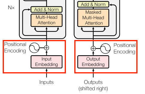
嵌入和位置編碼層

編碼器和解碼器的輸入都使用相同的嵌入和位置編碼邏輯。

嵌入和位置編碼層

給定權杖序列，輸入權杖 (葡萄牙文) 和目標權杖 (英文) 都必須使用 tf.keras.layers.Embedding 層轉換為向量。

模型中使用的注意力層將其輸入視為一組沒有順序的向量。由於模型不包含任何循環或卷積層。它需要某種方式來識別字詞順序，否則它會將輸入序列視為詞袋實例，how are you、how you are、you how are 等等，都是無法區分的。

Transformer 會將「位置編碼」新增至嵌入向量。它使用一組不同頻率的正弦波和餘弦波 (跨序列)。根據定義，附近的元素將具有相似的位置編碼。

原始論文使用以下公式來計算位置編碼

\[\Large{PE_{(pos, 2i)} = \sin(pos / 10000^{2i / d_{model} })} \]

\[\Large{PE_{(pos, 2i+1)} = \cos(pos / 10000^{2i / d_{model} })} \]

def positional_encoding(length, depth):
  depth = depth/2

  positions = np.arange(length)[:, np.newaxis]     # (seq, 1)
  depths = np.arange(depth)[np.newaxis, :]/depth   # (1, depth)

  angle_rates = 1 / (10000**depths)         # (1, depth)
  angle_rads = positions * angle_rates      # (pos, depth)

  pos_encoding = np.concatenate(
      [np.sin(angle_rads), np.cos(angle_rads)],
      axis=-1) 

  return tf.cast(pos_encoding, dtype=tf.float32)

位置編碼函式是一疊正弦波和餘弦波，它們根據在嵌入向量深度方向上的位置，以不同的頻率振動。它們沿著位置軸振動。

pos_encoding = positional_encoding(length=2048, depth=512)

# Check the shape.
print(pos_encoding.shape)

# Plot the dimensions.
plt.pcolormesh(pos_encoding.numpy().T, cmap='RdBu')
plt.ylabel('Depth')
plt.xlabel('Position')
plt.colorbar()
plt.show()

根據定義，這些向量與沿位置軸附近的向量對齊良好。在下方，位置編碼向量已正規化，並且透過點積將位置 1000 的向量與所有其他向量進行比較

pos_encoding/=tf.norm(pos_encoding, axis=1, keepdims=True)
p = pos_encoding[1000]
dots = tf.einsum('pd,d -> p', pos_encoding, p)
plt.subplot(2,1,1)
plt.plot(dots)
plt.ylim([0,1])
plt.plot([950, 950, float('nan'), 1050, 1050],
         [0,1,float('nan'),0,1], color='k', label='Zoom')
plt.legend()
plt.subplot(2,1,2)
plt.plot(dots)
plt.xlim([950, 1050])
plt.ylim([0,1])

因此，使用它來建立 PositionEmbedding 層，該層會查詢權杖的嵌入向量並新增位置向量

class PositionalEmbedding(tf.keras.layers.Layer):
  def __init__(self, vocab_size, d_model):
    super().__init__()
    self.d_model = d_model
    self.embedding = tf.keras.layers.Embedding(vocab_size, d_model, mask_zero=True) 
    self.pos_encoding = positional_encoding(length=2048, depth=d_model)

  def compute_mask(self, *args, **kwargs):
    return self.embedding.compute_mask(*args, **kwargs)

  def call(self, x):
    length = tf.shape(x)[1]
    x = self.embedding(x)
    # This factor sets the relative scale of the embedding and positonal_encoding.
    x *= tf.math.sqrt(tf.cast(self.d_model, tf.float32))
    x = x + self.pos_encoding[tf.newaxis, :length, :]
    return x

embed_pt = PositionalEmbedding(vocab_size=tokenizers.pt.get_vocab_size().numpy(), d_model=512)
embed_en = PositionalEmbedding(vocab_size=tokenizers.en.get_vocab_size().numpy(), d_model=512)

pt_emb = embed_pt(pt)
en_emb = embed_en(en)

en_emb._keras_mask

新增和正規化

新增和正規化

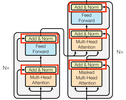
這些「新增和正規化」區塊散佈在整個模型中。每個區塊都結合了殘差連線，並透過 LayerNormalization 層執行結果。

組織程式碼最簡單的方式是圍繞這些殘差區塊。以下章節將為每個區塊定義自訂層類別。

包含殘差「新增和正規化」區塊是為了讓訓練有效率。殘差連線為梯度提供直接路徑 (並確保向量透過注意力層更新而不是取代)，而正規化則維持輸出合理的規模。

基本注意力層

注意力層遍佈整個模型使用。這些層都相同，只是注意力機制的設定方式不同。每個層都包含 layers.MultiHeadAttention、layers.LayerNormalization 和 layers.Add。

基本注意力層

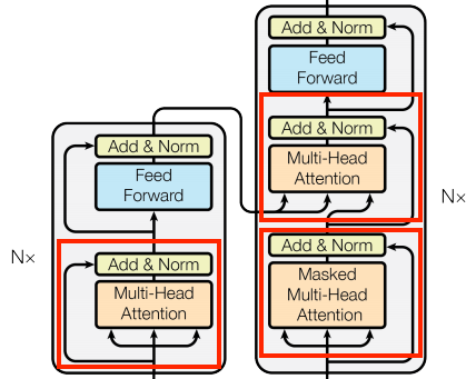
若要實作這些注意力層，請從僅包含元件層的簡單基底類別開始。每個用例都將實作為子類別。以這種方式編寫的程式碼會稍多一些，但可以保持意圖清晰。

class BaseAttention(tf.keras.layers.Layer):
  def __init__(self, **kwargs):
    super().__init__()
    self.mha = tf.keras.layers.MultiHeadAttention(**kwargs)
    self.layernorm = tf.keras.layers.LayerNormalization()
    self.add = tf.keras.layers.Add()

注意力機制複習

在您深入瞭解每個用法的細節之前，以下快速複習注意力機制的工作方式

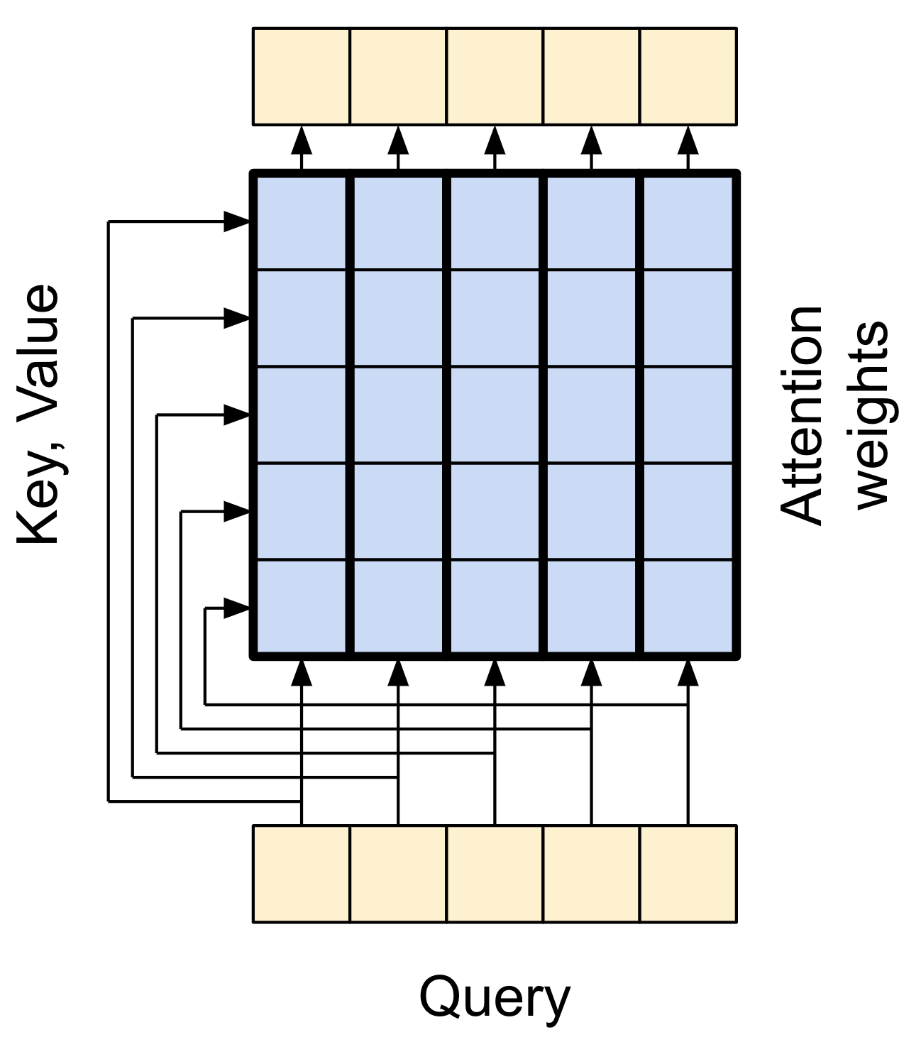
基本注意力層

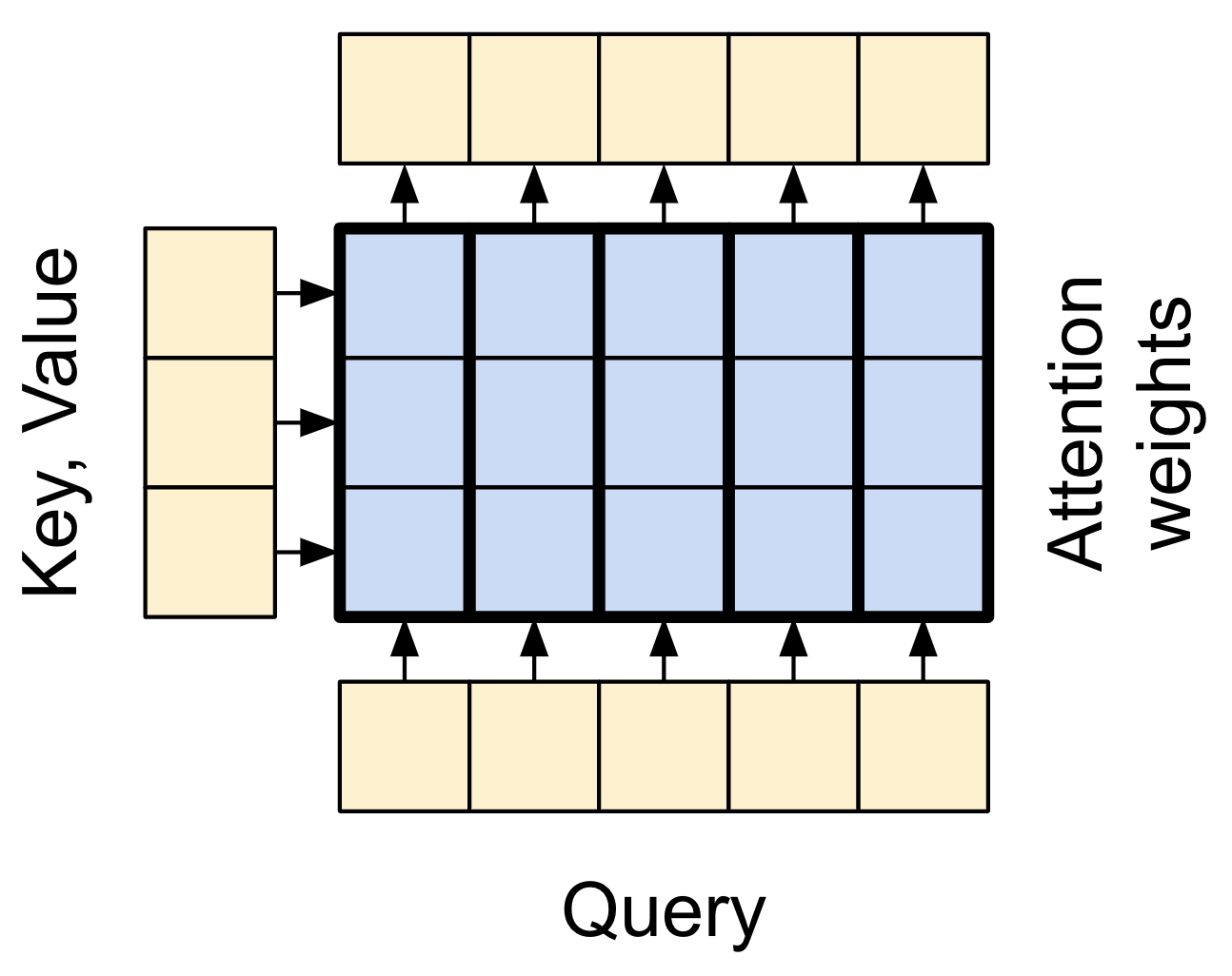
有兩個輸入

1. 查詢序列；正在處理的序列；執行注意力的序列 (底部)。
2. 脈絡序列；正在注意的序列 (左側)。

輸出具有與查詢序列相同的形狀。

常見的比較是此運算類似於字典查詢。模糊、可微分、向量化的字典查詢。

以下是一般的 Python 字典，其中 3 個鍵和 3 個值正傳遞單個查詢。

d = {'color': 'blue', 'age': 22, 'type': 'pickup'}
result = d['color']

• query 是您嘗試尋找的內容。
• key 是字典擁有的資訊類型。
• value 是該資訊。

當您在一般字典中查詢 query 時，字典會找到相符的 key，並傳回其關聯的 value。query 要麼具有相符的 key，要麼沒有。您可以想像一個模糊字典，其中鍵不必完全匹配。如果您在上面的字典中查詢 d["species"]，您可能希望它傳回 "pickup"，因為這是查詢的最佳匹配。

注意力層執行類似這樣的模糊查詢，但它不僅僅是尋找最佳鍵。它會根據 query 與每個 key 的匹配程度來組合 value。

它是如何運作的？在注意力層中，query、key 和 value 各自都是向量。注意力層不是執行雜湊查詢，而是組合 query 和 key 向量以判斷它們的匹配程度，即「注意力分數」。該層會傳回所有 value 的平均值，並依「注意力分數」加權。

查詢序列的每個位置都提供一個 query 向量。脈絡序列充當字典。脈絡序列中的每個位置都提供一個 key 和 value 向量。輸入向量不會直接使用，layers.MultiHeadAttention 層包含 layers.Dense 層，用於在使用輸入向量之前投射它們。

跨注意力層

Transformer 的字面中心是跨注意力層。此層連接編碼器和解碼器。此層是模型中最直接的注意力機制用法，它執行與使用注意力機制的 NMT 教學課程中注意力區塊相同的任務。

跨注意力層

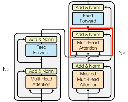
若要實作此功能，您可以在呼叫 mha 層時，將目標序列 x 作為 query，並將 context 序列作為 key/value 傳遞

class CrossAttention(BaseAttention):
  def call(self, x, context):
    attn_output, attn_scores = self.mha(
        query=x,
        key=context,
        value=context,
        return_attention_scores=True)

    # Cache the attention scores for plotting later.
    self.last_attn_scores = attn_scores

    x = self.add([x, attn_output])
    x = self.layernorm(x)

    return x

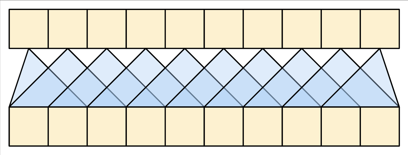
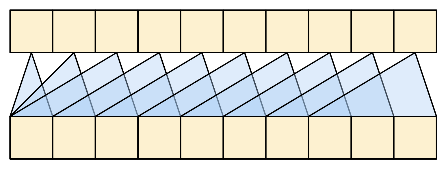
下方的漫畫顯示資訊如何流經此層。這些欄代表脈絡序列上的加權總和。

為了簡單起見，未顯示殘差連線。

跨注意力層

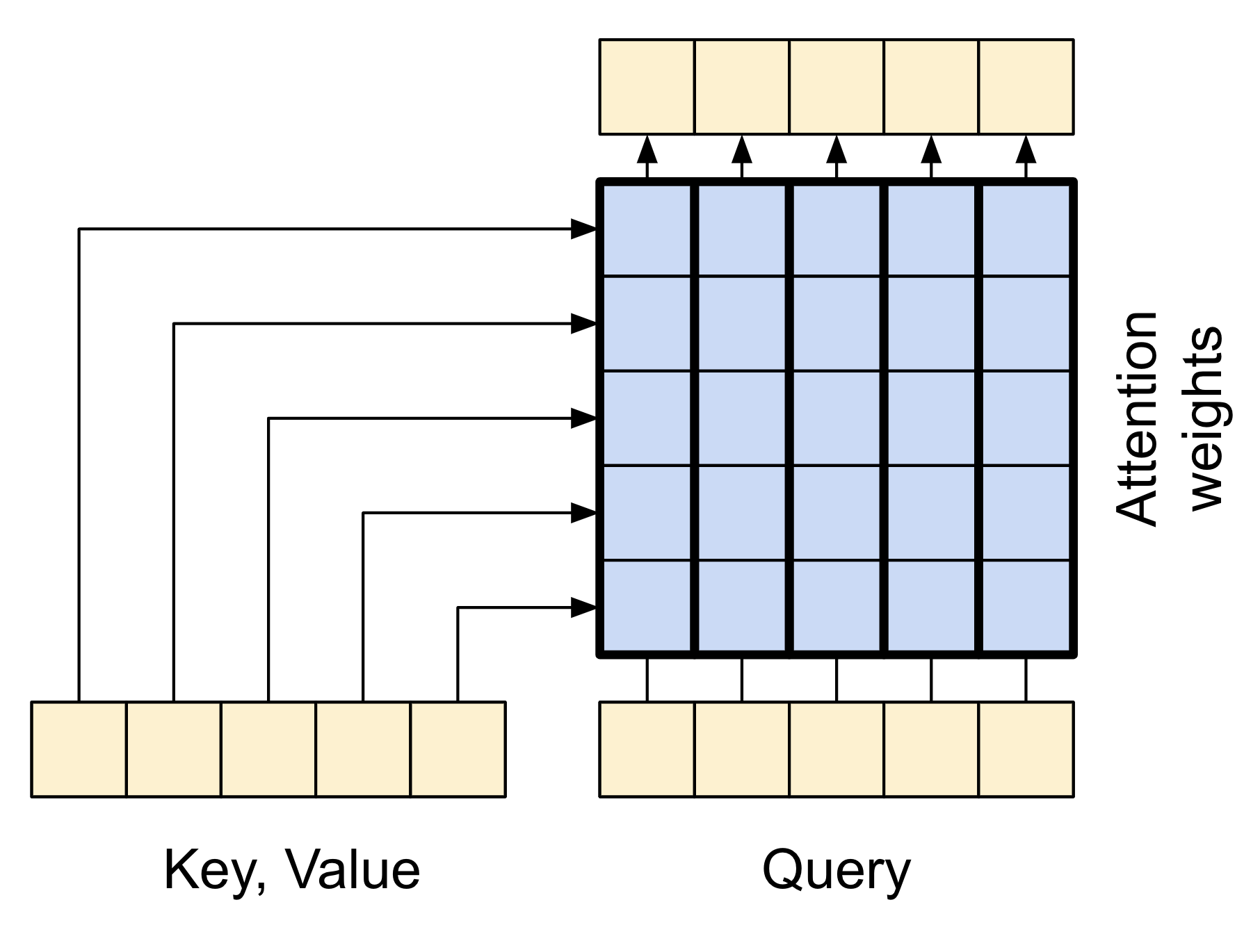
輸出長度是 query 序列的長度，而不是脈絡 key/value 序列的長度。

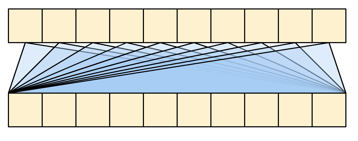
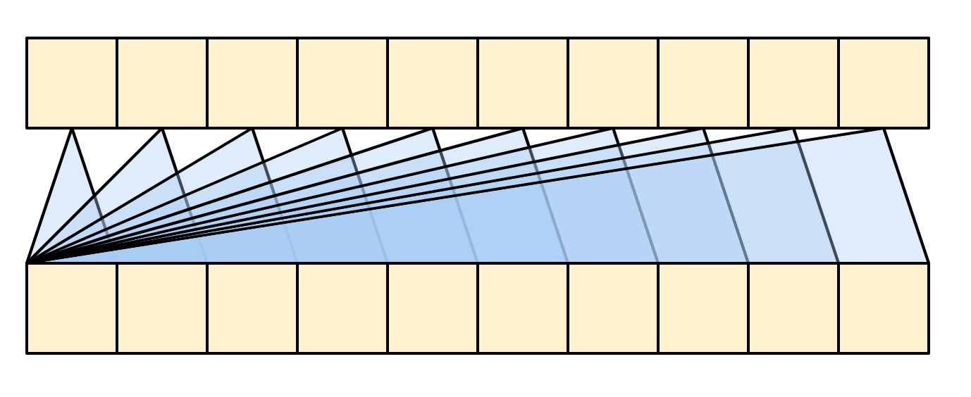
下圖進一步簡化了該圖表。無需繪製整個「注意力權重」矩陣。重點在於每個 query 位置都可以看到脈絡中的所有 key/value 組，但查詢之間不會交換任何資訊。

每個查詢都會看到整個脈絡。

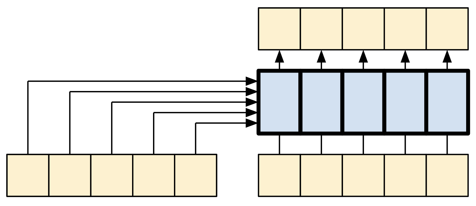
在範例輸入上進行測試執行

sample_ca = CrossAttention(num_heads=2, key_dim=512)

print(pt_emb.shape)
print(en_emb.shape)
print(sample_ca(en_emb, pt_emb).shape)

全域自我注意力層

此層負責處理脈絡序列，並沿其長度傳播資訊

全域自我注意力層

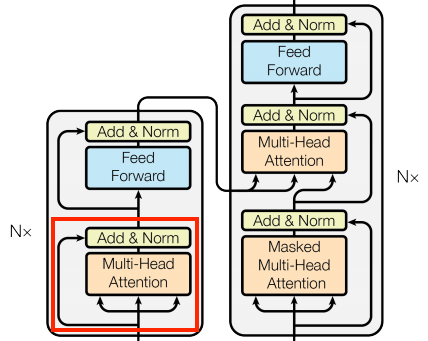
由於脈絡序列在產生翻譯時是固定的，因此允許資訊雙向流動。

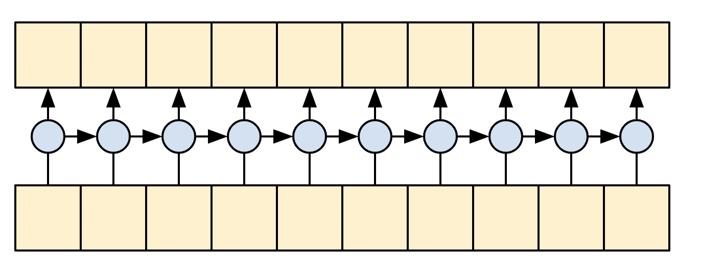
在 Transformer 和自我注意力機制之前，模型通常使用 RNN 或 CNN 來執行此任務

雙向 RNN 和 CNN

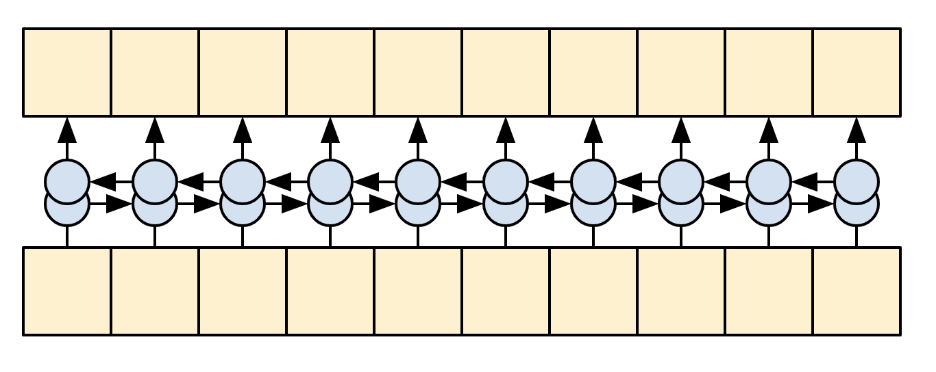
RNN 和 CNN 有其限制。

• RNN 允許資訊一直流過序列，但它需要通過許多處理步驟才能到達那裡 (限制梯度流)。這些 RNN 步驟必須循序執行，因此 RNN 較無法利用現代平行裝置。
• 在 CNN 中，每個位置都可以平行處理，但它只提供有限的感受野。感受野僅隨著 CNN 層數線性成長。您需要堆疊多個卷積層才能跨序列傳輸資訊 (Wavenet 透過使用擴張卷積來減少此問題)。

另一方面，全域自我注意力層讓每個序列元素都能直接存取每個其他序列元素，只需幾個運算，並且所有輸出都可以平行計算。

若要實作此層，您只需要將目標序列 x 同時作為 query 和 value 引數傳遞給 mha 層即可

class GlobalSelfAttention(BaseAttention):
  def call(self, x):
    attn_output = self.mha(
        query=x,
        value=x,
        key=x)
    x = self.add([x, attn_output])
    x = self.layernorm(x)
    return x

sample_gsa = GlobalSelfAttention(num_heads=2, key_dim=512)

print(pt_emb.shape)
print(sample_gsa(pt_emb).shape)

與之前相同的樣式，您可以像這樣繪製它

全域自我注意力層

同樣，為了清楚起見，省略了殘差連線。

像這樣繪製它更簡潔，而且同樣準確

全域自我注意力層

因果自我注意力層

此層為輸出序列執行與全域自我注意力層類似的工作

因果自我注意力層

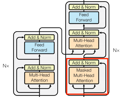
這需要與編碼器的全域自我注意力層區別處理。

如同文字生成教學課程和具備注意力機制的 NMT 教學課程，Transformer 是一種「自迴歸」模型：它們一次產生一個文字符元，並將該輸出回饋到輸入中。為了使此過程有效率，這些模型確保每個序列元素的輸出僅取決於先前的序列元素；這些模型是「因果關係」。

單向 RNN 依定義具有因果關係。若要建立因果關係迴旋積，您只需填充輸入並移動輸出，使其正確對齊 (使用 layers.Conv1D(padding='causal'))。

因果關係 RNN 和 CNN

因果關係模型在兩個方面具有效率

1. 在訓練中，它讓您在僅執行模型一次的情況下，即可計算輸出序列中每個位置的損失。
2. 在推論期間，對於每個新產生的符元，您只需要計算其輸出，先前序列元素的輸出可以重複使用。
   • 對於 RNN，您只需要 RNN 狀態來考量先前的計算 (將 return_state=True 傳遞至 RNN 層的建構函式)。
   • 對於 CNN，您需要遵循 Fast Wavenet 的方法

若要建構因果關係自我注意力層，您需要在計算注意力分數和加總注意力 value 時使用適當的遮罩。

如果您在呼叫 MultiHeadAttention 層時傳遞 use_causal_mask = True，則會自動處理此問題

class CausalSelfAttention(BaseAttention):
  def call(self, x):
    attn_output = self.mha(
        query=x,
        value=x,
        key=x,
        use_causal_mask = True)
    x = self.add([x, attn_output])
    x = self.layernorm(x)
    return x

因果關係遮罩確保每個位置僅能存取位於其之前的位置

因果自我注意力層

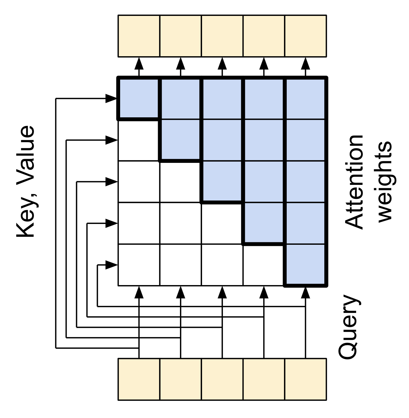
同樣地，為了簡化起見，省略了殘差連接。

此層更精簡的表示法會是

因果自我注意力層

測試此層

sample_csa = CausalSelfAttention(num_heads=2, key_dim=512)

print(en_emb.shape)
print(sample_csa(en_emb).shape)

早期序列元素的輸出不取決於後續元素，因此在套用此層之前或之後修剪元素應該沒有差別

out1 = sample_csa(embed_en(en[:, :3])) 
out2 = sample_csa(embed_en(en))[:, :3]

tf.reduce_max(abs(out1 - out2)).numpy()

前饋網路

Transformer 也包含編碼器和解碼器中的點狀前饋網路

前饋網路

此網路包含兩個線性層 (tf.keras.layers.Dense)，中間有一個 ReLU 啟動層和一個 dropout 層。與注意力層一樣，此處的程式碼也包含殘差連接和正規化

class FeedForward(tf.keras.layers.Layer):
  def __init__(self, d_model, dff, dropout_rate=0.1):
    super().__init__()
    self.seq = tf.keras.Sequential([
      tf.keras.layers.Dense(dff, activation='relu'),
      tf.keras.layers.Dense(d_model),
      tf.keras.layers.Dropout(dropout_rate)
    ])
    self.add = tf.keras.layers.Add()
    self.layer_norm = tf.keras.layers.LayerNormalization()

  def call(self, x):
    x = self.add([x, self.seq(x)])
    x = self.layer_norm(x) 
    return x

測試此層，輸出與輸入的形狀相同

sample_ffn = FeedForward(512, 2048)

print(en_emb.shape)
print(sample_ffn(en_emb).shape)

編碼器層

編碼器包含 N 個編碼器層的堆疊。其中每個 EncoderLayer 都包含 GlobalSelfAttention 和 FeedForward 層

編碼器層

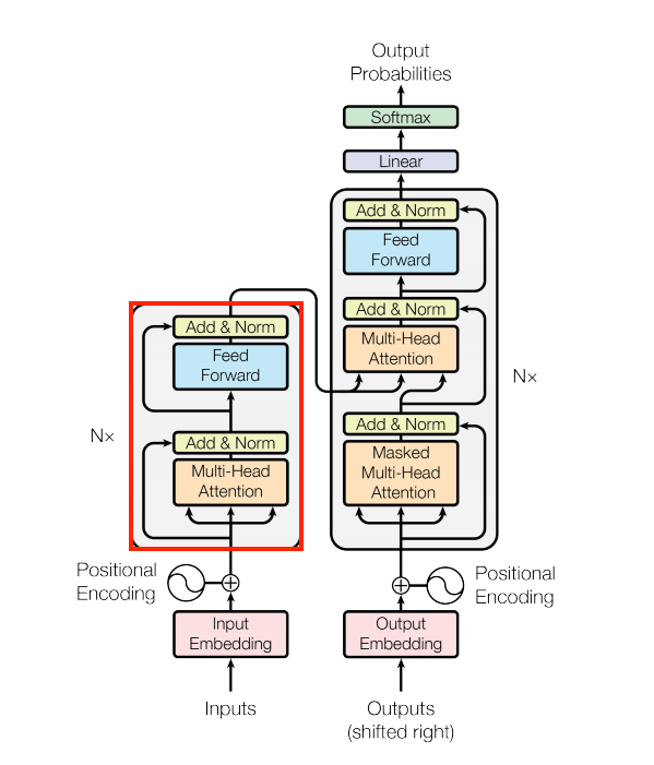
以下是 EncoderLayer 的定義

class EncoderLayer(tf.keras.layers.Layer):
  def __init__(self,*, d_model, num_heads, dff, dropout_rate=0.1):
    super().__init__()

    self.self_attention = GlobalSelfAttention(
        num_heads=num_heads,
        key_dim=d_model,
        dropout=dropout_rate)

    self.ffn = FeedForward(d_model, dff)

  def call(self, x):
    x = self.self_attention(x)
    x = self.ffn(x)
    return x

以及快速測試，輸出將具有與輸入相同的形狀

sample_encoder_layer = EncoderLayer(d_model=512, num_heads=8, dff=2048)

print(pt_emb.shape)
print(sample_encoder_layer(pt_emb).shape)

編碼器

接下來建構編碼器。

編碼器

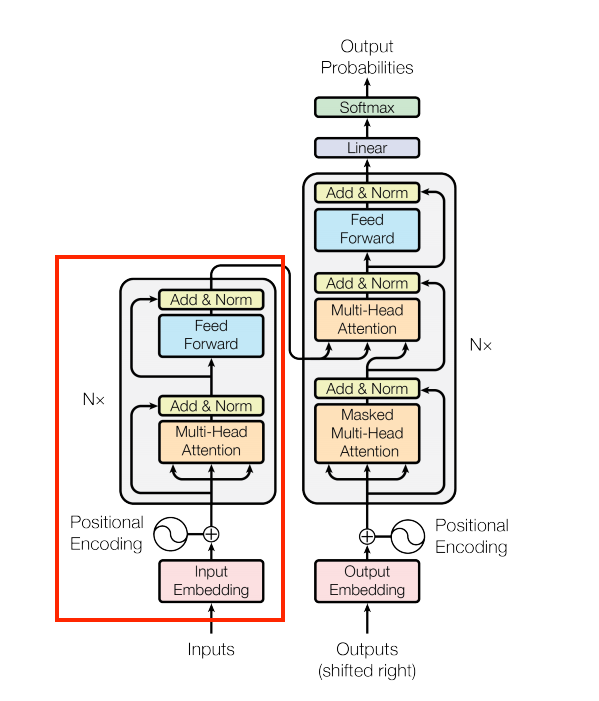
編碼器包含

• 輸入端的 PositionalEmbedding 層。
• EncoderLayer 層的堆疊。

class Encoder(tf.keras.layers.Layer):
  def __init__(self, *, num_layers, d_model, num_heads,
               dff, vocab_size, dropout_rate=0.1):
    super().__init__()

    self.d_model = d_model
    self.num_layers = num_layers

    self.pos_embedding = PositionalEmbedding(
        vocab_size=vocab_size, d_model=d_model)

    self.enc_layers = [
        EncoderLayer(d_model=d_model,
                     num_heads=num_heads,
                     dff=dff,
                     dropout_rate=dropout_rate)
        for _ in range(num_layers)]
    self.dropout = tf.keras.layers.Dropout(dropout_rate)

  def call(self, x):
    # `x` is token-IDs shape: (batch, seq_len)
    x = self.pos_embedding(x)  # Shape `(batch_size, seq_len, d_model)`.

    # Add dropout.
    x = self.dropout(x)

    for i in range(self.num_layers):
      x = self.enc_layers[i](x)

    return x  # Shape `(batch_size, seq_len, d_model)`.

測試編碼器

# Instantiate the encoder.
sample_encoder = Encoder(num_layers=4,
                         d_model=512,
                         num_heads=8,
                         dff=2048,
                         vocab_size=8500)

sample_encoder_output = sample_encoder(pt, training=False)

# Print the shape.
print(pt.shape)
print(sample_encoder_output.shape)  # Shape `(batch_size, input_seq_len, d_model)`.

解碼器層

解碼器的堆疊稍微複雜一些，每個 DecoderLayer 都包含 CausalSelfAttention、CrossAttention 和 FeedForward 層

解碼器層

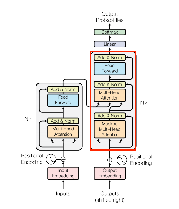
class DecoderLayer(tf.keras.layers.Layer):
  def __init__(self,
               *,
               d_model,
               num_heads,
               dff,
               dropout_rate=0.1):
    super(DecoderLayer, self).__init__()

    self.causal_self_attention = CausalSelfAttention(
        num_heads=num_heads,
        key_dim=d_model,
        dropout=dropout_rate)

    self.cross_attention = CrossAttention(
        num_heads=num_heads,
        key_dim=d_model,
        dropout=dropout_rate)

    self.ffn = FeedForward(d_model, dff)

  def call(self, x, context):
    x = self.causal_self_attention(x=x)
    x = self.cross_attention(x=x, context=context)

    # Cache the last attention scores for plotting later
    self.last_attn_scores = self.cross_attention.last_attn_scores

    x = self.ffn(x)  # Shape `(batch_size, seq_len, d_model)`.
    return x

測試解碼器層

sample_decoder_layer = DecoderLayer(d_model=512, num_heads=8, dff=2048)

sample_decoder_layer_output = sample_decoder_layer(
    x=en_emb, context=pt_emb)

print(en_emb.shape)
print(pt_emb.shape)
print(sample_decoder_layer_output.shape)  # `(batch_size, seq_len, d_model)`

解碼器

與 Encoder 類似，Decoder 包含 PositionalEmbedding 和 DecoderLayer 的堆疊

嵌入和位置編碼層

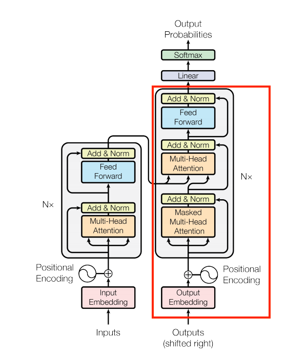
透過擴充 tf.keras.layers.Layer 來定義解碼器

class Decoder(tf.keras.layers.Layer):
  def __init__(self, *, num_layers, d_model, num_heads, dff, vocab_size,
               dropout_rate=0.1):
    super(Decoder, self).__init__()

    self.d_model = d_model
    self.num_layers = num_layers

    self.pos_embedding = PositionalEmbedding(vocab_size=vocab_size,
                                             d_model=d_model)
    self.dropout = tf.keras.layers.Dropout(dropout_rate)
    self.dec_layers = [
        DecoderLayer(d_model=d_model, num_heads=num_heads,
                     dff=dff, dropout_rate=dropout_rate)
        for _ in range(num_layers)]

    self.last_attn_scores = None

  def call(self, x, context):
    # `x` is token-IDs shape (batch, target_seq_len)
    x = self.pos_embedding(x)  # (batch_size, target_seq_len, d_model)

    x = self.dropout(x)

    for i in range(self.num_layers):
      x  = self.dec_layers[i](x, context)

    self.last_attn_scores = self.dec_layers[-1].last_attn_scores

    # The shape of x is (batch_size, target_seq_len, d_model).
    return x

測試解碼器

# Instantiate the decoder.
sample_decoder = Decoder(num_layers=4,
                         d_model=512,
                         num_heads=8,
                         dff=2048,
                         vocab_size=8000)

output = sample_decoder(
    x=en,
    context=pt_emb)

# Print the shapes.
print(en.shape)
print(pt_emb.shape)
print(output.shape)

sample_decoder.last_attn_scores.shape  # (batch, heads, target_seq, input_seq)

建立 Transformer 編碼器和解碼器之後，現在可以建構 Transformer 模型並進行訓練。

Transformer

您現在有 Encoder 和 Decoder。若要完成 Transformer 模型，您需要將它們放在一起，並新增最終線性 (Dense) 層，將每個位置的結果向量轉換為輸出符元機率。

解碼器的輸出是最終線性層的輸入。

Transformer

在 Encoder 和 Decoder 中都只有一層的 Transformer 看起來幾乎與RNN+注意力機制教學課程中的模型完全相同。多層 Transformer 具有更多層，但從根本上來說做的是相同的事情。

單層 Transformer	4 層 Transformer
RNN+注意力機制模型

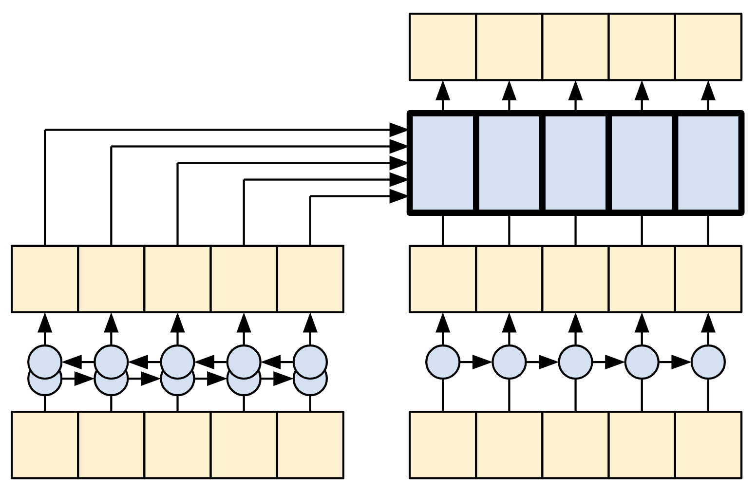
透過擴充 tf.keras.Model 來建立 Transformer

class Transformer(tf.keras.Model):
  def __init__(self, *, num_layers, d_model, num_heads, dff,
               input_vocab_size, target_vocab_size, dropout_rate=0.1):
    super().__init__()
    self.encoder = Encoder(num_layers=num_layers, d_model=d_model,
                           num_heads=num_heads, dff=dff,
                           vocab_size=input_vocab_size,
                           dropout_rate=dropout_rate)

    self.decoder = Decoder(num_layers=num_layers, d_model=d_model,
                           num_heads=num_heads, dff=dff,
                           vocab_size=target_vocab_size,
                           dropout_rate=dropout_rate)

    self.final_layer = tf.keras.layers.Dense(target_vocab_size)

  def call(self, inputs):
    # To use a Keras model with `.fit` you must pass all your inputs in the
    # first argument.
    context, x  = inputs

    context = self.encoder(context)  # (batch_size, context_len, d_model)

    x = self.decoder(x, context)  # (batch_size, target_len, d_model)

    # Final linear layer output.
    logits = self.final_layer(x)  # (batch_size, target_len, target_vocab_size)

    try:
      # Drop the keras mask, so it doesn't scale the losses/metrics.
      # b/250038731
      del logits._keras_mask
    except AttributeError:
      pass

    # Return the final output and the attention weights.
    return logits

超參數

為了使此範例保持小巧且相對快速，已減少層數 (num_layers)、嵌入的維度 (d_model) 和 FeedForward 層的內部維度 (dff)。

原始 Transformer 論文中描述的基本模型使用 num_layers=6、d_model=512 和 dff=2048。

自我注意力機制的頭數保持不變 (num_heads=8)。

num_layers = 4
d_model = 128
dff = 512
num_heads = 8
dropout_rate = 0.1

試用看看

例項化 Transformer 模型

transformer = Transformer(
    num_layers=num_layers,
    d_model=d_model,
    num_heads=num_heads,
    dff=dff,
    input_vocab_size=tokenizers.pt.get_vocab_size().numpy(),
    target_vocab_size=tokenizers.en.get_vocab_size().numpy(),
    dropout_rate=dropout_rate)

測試看看

output = transformer((pt, en))

print(en.shape)
print(pt.shape)
print(output.shape)

attn_scores = transformer.decoder.dec_layers[-1].last_attn_scores
print(attn_scores.shape)  # (batch, heads, target_seq, input_seq)

列印模型摘要

transformer.summary()

訓練

現在可以準備模型並開始訓練。

設定最佳化工具

根據原始 Transformer 論文中的公式，使用具有自訂學習率排程器的 Adam 最佳化工具。

\[\Large{lrate = d_{model}^{-0.5} * \min(step{\_}num^{-0.5}, step{\_}num \cdot warmup{\_}steps^{-1.5})}\]

class CustomSchedule(tf.keras.optimizers.schedules.LearningRateSchedule):
  def __init__(self, d_model, warmup_steps=4000):
    super().__init__()

    self.d_model = d_model
    self.d_model = tf.cast(self.d_model, tf.float32)

    self.warmup_steps = warmup_steps

  def __call__(self, step):
    step = tf.cast(step, dtype=tf.float32)
    arg1 = tf.math.rsqrt(step)
    arg2 = step * (self.warmup_steps ** -1.5)

    return tf.math.rsqrt(self.d_model) * tf.math.minimum(arg1, arg2)

例項化最佳化工具 (在此範例中為 tf.keras.optimizers.Adam)

learning_rate = CustomSchedule(d_model)

optimizer = tf.keras.optimizers.Adam(learning_rate, beta_1=0.9, beta_2=0.98,
                                     epsilon=1e-9)

測試自訂學習率排程器

plt.plot(learning_rate(tf.range(40000, dtype=tf.float32)))
plt.ylabel('Learning Rate')
plt.xlabel('Train Step')

設定損失和指標

由於目標序列已填充，因此在計算損失時套用填充遮罩非常重要。使用交叉熵損失函數 (tf.keras.losses.SparseCategoricalCrossentropy)

def masked_loss(label, pred):
  mask = label != 0
  loss_object = tf.keras.losses.SparseCategoricalCrossentropy(
    from_logits=True, reduction='none')
  loss = loss_object(label, pred)

  mask = tf.cast(mask, dtype=loss.dtype)
  loss *= mask

  loss = tf.reduce_sum(loss)/tf.reduce_sum(mask)
  return loss


def masked_accuracy(label, pred):
  pred = tf.argmax(pred, axis=2)
  label = tf.cast(label, pred.dtype)
  match = label == pred

  mask = label != 0

  match = match & mask

  match = tf.cast(match, dtype=tf.float32)
  mask = tf.cast(mask, dtype=tf.float32)
  return tf.reduce_sum(match)/tf.reduce_sum(mask)

訓練模型

所有元件都準備就緒後，使用 model.compile 設定訓練程序，然後使用 model.fit 執行。

transformer.compile(
    loss=masked_loss,
    optimizer=optimizer,
    metrics=[masked_accuracy])

transformer.fit(train_batches,
                epochs=20,
                validation_data=val_batches)

執行推論

您現在可以透過執行翻譯來測試模型。以下步驟用於推論

• 使用葡萄牙文符元化工具 (tokenizers.pt) 編碼輸入句子。這是編碼器輸入。
• 解碼器輸入會初始化為 [START] 符元。
• 計算填充遮罩和前瞻遮罩。
• 然後 decoder 會透過查看 encoder output 和其自身的輸出 (自我注意力機制) 來輸出預測。
• 將預測的符元串連到解碼器輸入，並將其傳遞至解碼器。
• 在此方法中，解碼器會根據其先前預測的符元來預測下一個符元。

透過子類別化 tf.Module 來定義 Translator 類別

class Translator(tf.Module):
  def __init__(self, tokenizers, transformer):
    self.tokenizers = tokenizers
    self.transformer = transformer

  def __call__(self, sentence, max_length=MAX_TOKENS):
    # The input sentence is Portuguese, hence adding the `[START]` and `[END]` tokens.
    assert isinstance(sentence, tf.Tensor)
    if len(sentence.shape) == 0:
      sentence = sentence[tf.newaxis]

    sentence = self.tokenizers.pt.tokenize(sentence).to_tensor()

    encoder_input = sentence

    # As the output language is English, initialize the output with the
    # English `[START]` token.
    start_end = self.tokenizers.en.tokenize([''])[0]
    start = start_end[0][tf.newaxis]
    end = start_end[1][tf.newaxis]

    # `tf.TensorArray` is required here (instead of a Python list), so that the
    # dynamic-loop can be traced by `tf.function`.
    output_array = tf.TensorArray(dtype=tf.int64, size=0, dynamic_size=True)
    output_array = output_array.write(0, start)

    for i in tf.range(max_length):
      output = tf.transpose(output_array.stack())
      predictions = self.transformer([encoder_input, output], training=False)

      # Select the last token from the `seq_len` dimension.
      predictions = predictions[:, -1:, :]  # Shape `(batch_size, 1, vocab_size)`.

      predicted_id = tf.argmax(predictions, axis=-1)

      # Concatenate the `predicted_id` to the output which is given to the
      # decoder as its input.
      output_array = output_array.write(i+1, predicted_id[0])

      if predicted_id == end:
        break

    output = tf.transpose(output_array.stack())
    # The output shape is `(1, tokens)`.
    text = tokenizers.en.detokenize(output)[0]  # Shape: `()`.

    tokens = tokenizers.en.lookup(output)[0]

    # `tf.function` prevents us from using the attention_weights that were
    # calculated on the last iteration of the loop.
    # So, recalculate them outside the loop.
    self.transformer([encoder_input, output[:,:-1]], training=False)
    attention_weights = self.transformer.decoder.last_attn_scores

    return text, tokens, attention_weights

建立此 Translator 類別的例項，並試用幾次

translator = Translator(tokenizers, transformer)

def print_translation(sentence, tokens, ground_truth):
  print(f'{"Input:":15s}: {sentence}')
  print(f'{"Prediction":15s}: {tokens.numpy().decode("utf-8")}')
  print(f'{"Ground truth":15s}: {ground_truth}')

範例 1

sentence = 'este é um problema que temos que resolver.'
ground_truth = 'this is a problem we have to solve .'

translated_text, translated_tokens, attention_weights = translator(
    tf.constant(sentence))
print_translation(sentence, translated_text, ground_truth)

範例 2

sentence = 'os meus vizinhos ouviram sobre esta ideia.'
ground_truth = 'and my neighboring homes heard about this idea .'

translated_text, translated_tokens, attention_weights = translator(
    tf.constant(sentence))
print_translation(sentence, translated_text, ground_truth)

範例 3

sentence = 'vou então muito rapidamente partilhar convosco algumas histórias de algumas coisas mágicas que aconteceram.'
ground_truth = "so i'll just share with you some stories very quickly of some magical things that have happened."

translated_text, translated_tokens, attention_weights = translator(
    tf.constant(sentence))
print_translation(sentence, translated_text, ground_truth)

建立注意力機制圖

您在上一個章節中建立的 Translator 類別會傳回注意力機制熱圖的字典，您可以使用這些熱圖來視覺化模型的內部運作。

例如

sentence = 'este é o primeiro livro que eu fiz.'
ground_truth = "this is the first book i've ever done."

translated_text, translated_tokens, attention_weights = translator(
    tf.constant(sentence))
print_translation(sentence, translated_text, ground_truth)

建立在產生符元時繪製注意力機制的函式

def plot_attention_head(in_tokens, translated_tokens, attention):
  # The model didn't generate `<START>` in the output. Skip it.
  translated_tokens = translated_tokens[1:]

  ax = plt.gca()
  ax.matshow(attention)
  ax.set_xticks(range(len(in_tokens)))
  ax.set_yticks(range(len(translated_tokens)))

  labels = [label.decode('utf-8') for label in in_tokens.numpy()]
  ax.set_xticklabels(
      labels, rotation=90)

  labels = [label.decode('utf-8') for label in translated_tokens.numpy()]
  ax.set_yticklabels(labels)

head = 0
# Shape: `(batch=1, num_heads, seq_len_q, seq_len_k)`.
attention_heads = tf.squeeze(attention_weights, 0)
attention = attention_heads[head]
attention.shape

這些是輸入 (葡萄牙文) 符元

in_tokens = tf.convert_to_tensor([sentence])
in_tokens = tokenizers.pt.tokenize(in_tokens).to_tensor()
in_tokens = tokenizers.pt.lookup(in_tokens)[0]
in_tokens

這些是輸出 (英文翻譯) 符元

translated_tokens

plot_attention_head(in_tokens, translated_tokens, attention)

def plot_attention_weights(sentence, translated_tokens, attention_heads):
  in_tokens = tf.convert_to_tensor([sentence])
  in_tokens = tokenizers.pt.tokenize(in_tokens).to_tensor()
  in_tokens = tokenizers.pt.lookup(in_tokens)[0]

  fig = plt.figure(figsize=(16, 8))

  for h, head in enumerate(attention_heads):
    ax = fig.add_subplot(2, 4, h+1)

    plot_attention_head(in_tokens, translated_tokens, head)

    ax.set_xlabel(f'Head {h+1}')

  plt.tight_layout()
  plt.show()

plot_attention_weights(sentence,
                       translated_tokens,
                       attention_weights[0])

模型可以處理不熟悉的單字。'triceratops' 和 'encyclopédia' 都不在輸入資料集中，即使沒有共用詞彙，模型也會嘗試音譯它們。例如

sentence = 'Eu li sobre triceratops na enciclopédia.'
ground_truth = 'I read about triceratops in the encyclopedia.'

translated_text, translated_tokens, attention_weights = translator(
    tf.constant(sentence))
print_translation(sentence, translated_text, ground_truth)

plot_attention_weights(sentence, translated_tokens, attention_weights[0])

匯出模型

您已測試模型，且推論運作正常。接下來，您可以將其匯出為 tf.saved_model。若要進一步瞭解如何以 SavedModel 格式儲存及載入模型，請使用 本指南。

透過子類別化 tf.Module 子類別來建立名為 ExportTranslator 的類別，並在 __call__ 方法上使用 tf.function

class ExportTranslator(tf.Module):
  def __init__(self, translator):
    self.translator = translator

  @tf.function(input_signature=[tf.TensorSpec(shape=[], dtype=tf.string)])
  def __call__(self, sentence):
    (result,
     tokens,
     attention_weights) = self.translator(sentence, max_length=MAX_TOKENS)

    return result

在上述 tf.function 中，僅傳回輸出句子。由於 非嚴格執行 在 tf.function 中，因此永遠不會計算任何不必要的值。

將 translator 包裝在新建立的 ExportTranslator 中

translator = ExportTranslator(translator)

由於模型正在使用 tf.argmax 解碼預測，因此預測是決定性的。從其 SavedModel 重新載入的原始模型和模型應提供相同的預測

translator('este é o primeiro livro que eu fiz.').numpy()

tf.saved_model.save(translator, export_dir='translator')

reloaded = tf.saved_model.load('translator')

reloaded('este é o primeiro livro que eu fiz.').numpy()

結論

在本教學課程中，您學到了

• Transformer 及其在機器學習中的重要性
• 注意力機制、自我注意力機制和多頭注意力機制
• 具有嵌入的位置編碼
• 原始 Transformer 的編碼器-解碼器架構
• 自我注意力機制中的遮罩
• 如何將所有內容放在一起以翻譯文字

此架構的缺點如下

• 對於時間序列，時間步的輸出是從整個歷史記錄計算而來，而不僅僅是輸入和目前的隱藏狀態。這可能效率較低。
• 如果輸入具有時間/空間關係 (例如文字或圖片)，則必須新增一些位置編碼，否則模型實際上會看到詞袋。

如果您想練習，可以嘗試許多事情。例如

• 使用不同的資料集來訓練 Transformer。
• 透過變更超參數，從原始論文中建立「基本 Transformer」或「Transformer XL」組態。
• 使用此處定義的層來建立 BERT 的實作
• 使用集束搜尋以獲得更好的預測。

有各種以 Transformer 為基礎的模型，其中許多模型改進了 2017 年版的原始 Transformer，具有編碼器-解碼器、僅編碼器和僅解碼器架構。

以下研究出版品涵蓋了其中一些模型

• 「高效 Transformer：調查」 (Tay 等人，2022 年)
• 「Transformer 的正式演算法」 (Phuong 和 Hutter，2022 年)。
• T5 (「探索使用統一文字到文字 Transformer 進行遷移學習的限制」) (Raffel 等人，2019 年)

您可以在以下 Google 部落格文章中進一步瞭解其他模型

• PaLM.
• LaMDA
• MUM
• Reformer
• BERT

如果您有興趣研究以注意力機制為基礎的模型如何在自然語言處理以外的任務中應用，請查看以下資源

• Vision Transformer (ViT)：大規模影像辨識的 Transformer
• 使用 Transformer 的多任務多軌音樂轉錄 (MT3)
• 使用 AlphaCode 進行程式碼產生
• 使用多遊戲決策 Transformer 進行強化學習
• 使用 AlphaFold 進行蛋白質結構預測
• OptFormer：使用 Transformer 實現通用超參數最佳化