
|
|
|
 在 GitHub 上檢視 在 GitHub 上檢視
|
|
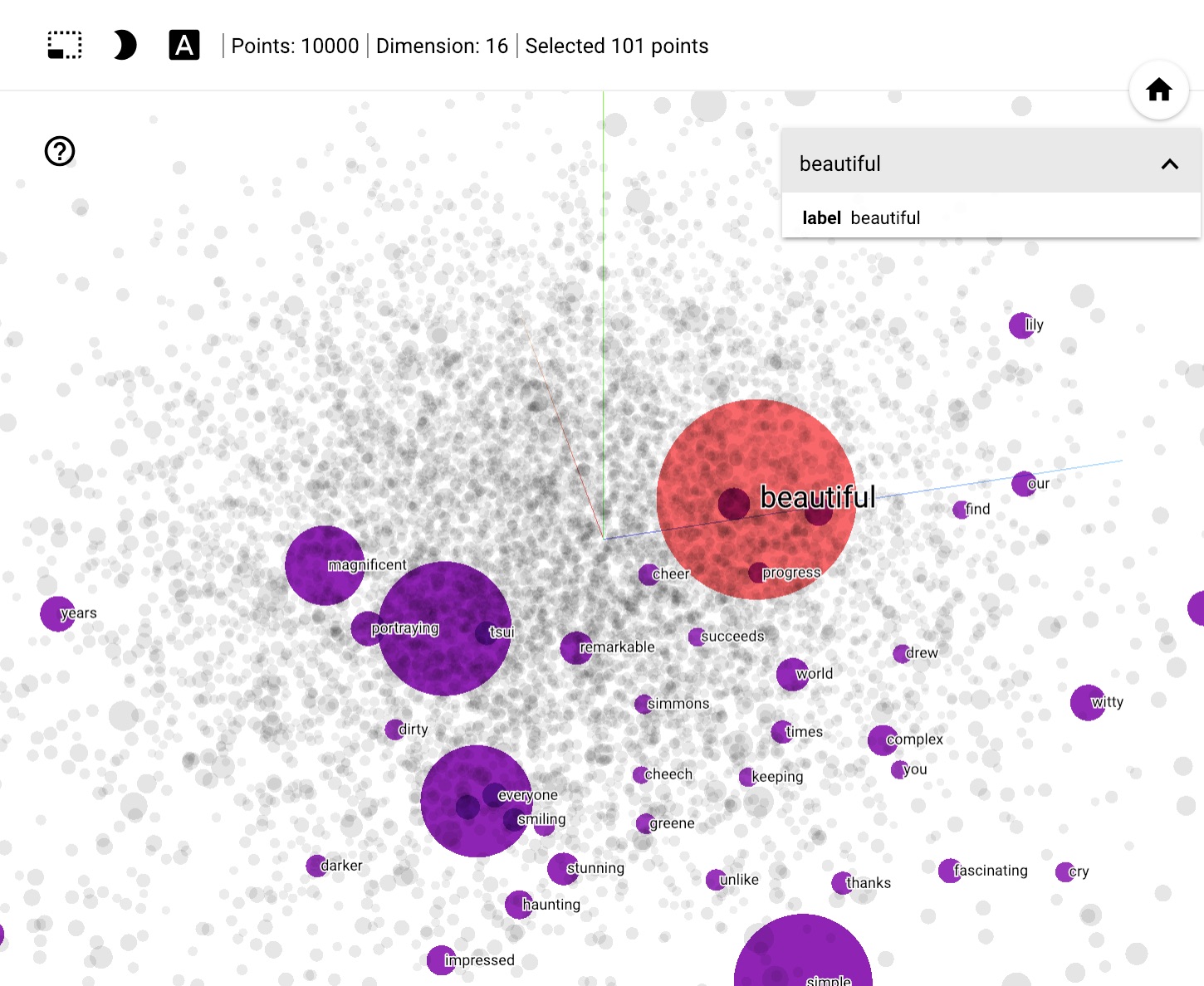
本教學課程簡介詞嵌入。您將使用簡單的 Keras 模型訓練自己的詞嵌入,以進行情感分類工作,然後在 Embedding Projector 中視覺化這些詞嵌入 (如下圖所示)。
將文字表示為數字
機器學習模型以向量 (數字陣列) 作為輸入。處理文字時,您必須做的第一件事是想出策略,將字串轉換為數字 (或將文字「向量化」),然後再饋送至模型。在本節中,您將了解三種策略。
獨熱編碼
第一個想法是,您可以對詞彙表中的每個字詞進行「獨熱」編碼。以句子「The cat sat on the mat」為例。此句子中的詞彙表 (或唯一字詞) 為 (cat、mat、on、sat、the)。為了表示每個字詞,您將建立一個長度等於詞彙表的零向量,然後在對應於該字詞的索引中放置一個 1。下圖顯示了此方法。
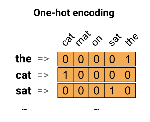
若要建立包含句子編碼的向量,您可以串連每個字詞的獨熱向量。
使用唯一數字編碼每個字詞
您可以嘗試的第二種方法是使用唯一數字編碼每個字詞。繼續上面的範例,您可以將 1 指派給「cat」,將 2 指派給「mat」,依此類推。然後,您可以將句子「The cat sat on the mat」編碼為密集向量,例如 [5, 1, 4, 3, 5, 2]。此方法效率很高。現在您擁有的是密集向量 (其中所有元素都是滿的),而不是稀疏向量。
但是,此方法有兩個缺點
整數編碼是任意的 (它無法捕捉字詞之間的任何關係)。
整數編碼對於模型來說可能難以解讀。例如,線性分類器會為每個特徵學習單一權重。由於任何兩個字詞的相似度與其編碼的相似度之間沒有關係,因此此特徵權重組合沒有意義。
詞嵌入
詞嵌入讓我們能夠使用有效率的密集表示法,其中相似的字詞具有相似的編碼。重要的是,您不必手動指定此編碼。嵌入是浮點值的密集向量 (向量的長度是您指定的參數)。嵌入的值不是手動指定,而是可訓練的參數 (模型在訓練期間學習到的權重,就像模型學習密集層的權重一樣)。常見的詞嵌入維度為 8 維 (適用於小型資料集) 到 1024 維 (適用於大型資料集)。維度較高的嵌入可以捕捉字詞之間更細微的關係,但需要更多資料才能學習。
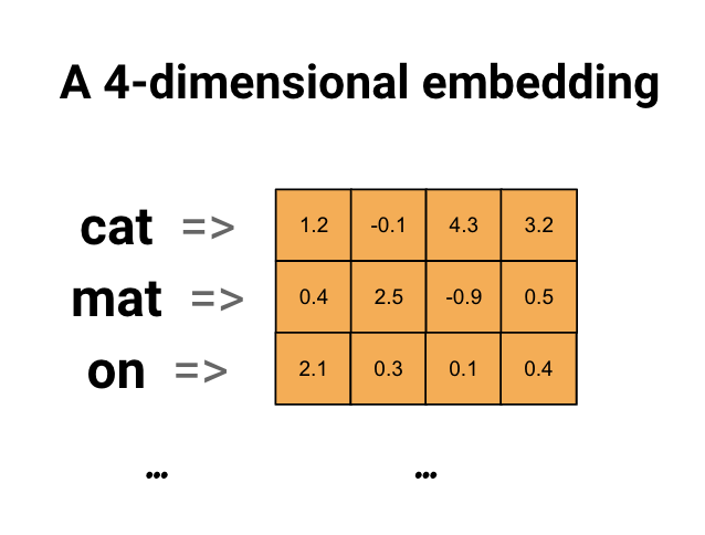
上方是詞嵌入的圖表。每個字詞都表示為 4 維浮點值向量。思考嵌入的另一種方式是「查閱表」。學習到這些權重後,您可以查閱表中對應的密集向量,藉此編碼每個字詞。
設定
import io
import os
import re
import shutil
import string
import tensorflow as tf

from tensorflow.keras import Sequential
from tensorflow.keras.layers import Dense, Embedding, GlobalAveragePooling1D
from tensorflow.keras.layers import TextVectorization
2023-11-16 14:12:20.714950: E external/local_xla/xla/stream_executor/cuda/cuda_dnn.cc:9261] Unable to register cuDNN factory: Attempting to register factory for plugin cuDNN when one has already been registered
2023-11-16 14:12:20.714992: E external/local_xla/xla/stream_executor/cuda/cuda_fft.cc:607] Unable to register cuFFT factory: Attempting to register factory for plugin cuFFT when one has already been registered
2023-11-16 14:12:20.716533: E external/local_xla/xla/stream_executor/cuda/cuda_blas.cc:1515] Unable to register cuBLAS factory: Attempting to register factory for plugin cuBLAS when one has already been registered
下載 IMDb 資料集
在本教學課程中,您將使用大型電影評論資料集。您將在此資料集上訓練情感分類器模型,並在此過程中從頭開始學習嵌入。如要進一步瞭解如何從頭開始載入資料集,請參閱載入文字教學課程。
使用 Keras 檔案公用程式下載資料集,並查看目錄。
url = "https://ai.stanford.edu/~amaas/data/sentiment/aclImdb_v1.tar.gz"

dataset = tf.keras.utils.get_file("aclImdb_v1.tar.gz", url,
                                  untar=True, cache_dir='.',
                                  cache_subdir='')

dataset_dir = os.path.join(os.path.dirname(dataset), 'aclImdb')
os.listdir(dataset_dir)
Downloading data from https://ai.stanford.edu/~amaas/data/sentiment/aclImdb_v1.tar.gz
84125825/84125825 [==============================] - 2s 0us/step
['train', 'README', 'imdb.vocab', 'test', 'imdbEr.txt']
查看 train/ 目錄。其中包含 pos 和 neg 資料夾,其中電影評論分別標示為正面和負面。您將使用 pos 和 neg 資料夾中的評論來訓練二元分類模型。
train_dir = os.path.join(dataset_dir, 'train')
os.listdir(train_dir)
['urls_unsup.txt',
 'unsupBow.feat',
 'unsup',
 'pos',
 'labeledBow.feat',
 'neg',
 'urls_pos.txt',
 'urls_neg.txt']
train 目錄還有其他資料夾,在建立訓練資料集之前應先移除這些資料夾。
remove_dir = os.path.join(train_dir, 'unsup')
shutil.rmtree(remove_dir)
接下來,使用 tf.keras.utils.text_dataset_from_directory 建立 tf.data.Dataset。您可以在此文字分類教學課程中進一步瞭解如何使用此公用程式。
使用 train 目錄建立訓練和驗證資料集,並將 20% 分割用於驗證。
batch_size = 1024
seed = 123
train_ds = tf.keras.utils.text_dataset_from_directory(
    'aclImdb/train', batch_size=batch_size, validation_split=0.2,
    subset='training', seed=seed)
val_ds = tf.keras.utils.text_dataset_from_directory(
    'aclImdb/train', batch_size=batch_size, validation_split=0.2,
    subset='validation', seed=seed)
Found 25000 files belonging to 2 classes.
Using 20000 files for training.
Found 25000 files belonging to 2 classes.
Using 5000 files for validation.
查看訓練資料集中的一些電影評論及其標籤 ((1: positive, 0: negative):正面,0:負面)。
for text_batch, label_batch in train_ds.take(1):
  for i in range(5):
    print(label_batch[i].numpy(), text_batch.numpy()[i])
0 b"Oh My God! Please, for the love of all that is holy, Do Not Watch This Movie! It it 82 minutes of my life I will never get back. Sure, I could have stopped watching half way through. But I thought it might get better. It Didn't. Anyone who actually enjoyed this movie is one seriously sick and twisted individual. No wonder us Australians/New Zealanders have a terrible reputation when it comes to making movies. Everything about this movie is horrible, from the acting to the editing. I don't even normally write reviews on here, but in this case I'll make an exception. I only wish someone had of warned me before I hired this catastrophe"
1 b'This movie is SOOOO funny!!! The acting is WONDERFUL, the Ramones are sexy, the jokes are subtle, and the plot is just what every high schooler dreams of doing to his/her school. I absolutely loved the soundtrack as well as the carefully placed cynicism. If you like monty python, You will love this film. This movie is a tad bit "grease"esk (without all the annoying songs). The songs that are sung are likable; you might even find yourself singing these songs once the movie is through. This musical ranks number two in musicals to me (second next to the blues brothers). But please, do not think of it as a musical per say; seeing as how the songs are so likable, it is hard to tell a carefully choreographed scene is taking place. I think of this movie as more of a comedy with undertones of romance. You will be reminded of what it was like to be a rebellious teenager; needless to say, you will be reminiscing of your old high school days after seeing this film. Highly recommended for both the family (since it is a very youthful but also for adults since there are many jokes that are funnier with age and experience.'
0 b"Alex D. Linz replaces Macaulay Culkin as the central figure in the third movie in the Home Alone empire. Four industrial spies acquire a missile guidance system computer chip and smuggle it through an airport inside a remote controlled toy car. Because of baggage confusion, grouchy Mrs. Hess (Marian Seldes) gets the car. She gives it to her neighbor, Alex (Linz), just before the spies turn up. The spies rent a house in order to burglarize each house in the neighborhood until they locate the car. Home alone with the chicken pox, Alex calls 911 each time he spots a theft in progress, but the spies always manage to elude the police while Alex is accused of making prank calls. The spies finally turn their attentions toward Alex, unaware that he has rigged devices to cleverly booby-trap his entire house. Home Alone 3 wasn't horrible, but probably shouldn't have been made, you can't just replace Macauley Culkin, Joe Pesci, or Daniel Stern. Home Alone 3 had some funny parts, but I don't like when characters are changed in a movie series, view at own risk."
0 b"There's a good movie lurking here, but this isn't it. The basic idea is good: to explore the moral issues that would face a group of young survivors of the apocalypse. But the logic is so muddled that it's impossible to get involved.<br /><br />For example, our four heroes are (understandably) paranoid about catching the mysterious airborne contagion that's wiped out virtually all of mankind. Yet they wear surgical masks some times, not others. Some times they're fanatical about wiping down with bleach any area touched by an infected person. Other times, they seem completely unconcerned.<br /><br />Worse, after apparently surviving some weeks or months in this new kill-or-be-killed world, these people constantly behave like total newbs. They don't bother accumulating proper equipment, or food. They're forever running out of fuel in the middle of nowhere. They don't take elementary precautions when meeting strangers. And after wading through the rotting corpses of the entire human race, they're as squeamish as sheltered debutantes. You have to constantly wonder how they could have survived this long... and even if they did, why anyone would want to make a movie about them.<br /><br />So when these dweebs stop to agonize over the moral dimensions of their actions, it's impossible to take their soul-searching seriously. Their actions would first have to make some kind of minimal sense.<br /><br />On top of all this, we must contend with the dubious acting abilities of Chris Pine. His portrayal of an arrogant young James T Kirk might have seemed shrewd, when viewed in isolation. But in Carriers he plays on exactly that same note: arrogant and boneheaded. It's impossible not to suspect that this constitutes his entire dramatic range.<br /><br />On the positive side, the film *looks* excellent. It's got an over-sharp, saturated look that really suits the southwestern US locale. But that can't save the truly feeble writing nor the paper-thin (and annoying) characters. Even if you're a fan of the end-of-the-world genre, you should save yourself the agony of watching Carriers."
0 b'I saw this movie at an actual movie theater (probably the \\(2.00 one) with my cousin and uncle. We were around 11 and 12, I guess, and really into scary movies. I remember being so excited to see it because my cool uncle let us pick the movie (and we probably never got to do that again!) and sooo disappointed afterwards!! Just boring and not scary. The only redeeming thing I can remember was Corky Pigeon from Silver Spoons, and that wasn\'t all that great, just someone I recognized. I\'ve seen bad movies before and this one has always stuck out in my mind as the worst. This was from what I can recall, one of the most boring, non-scary, waste of our collective \\)6, and a waste of film. I have read some of the reviews that say it is worth a watch and I say, "Too each his own", but I wouldn\'t even bother. Not even so bad it\'s good.'
設定資料集效能
這是載入資料時應使用的兩種重要方法,以確保 I/O 不會變成封鎖狀態。
.cache() 會在資料從磁碟載入後將資料保留在記憶體中。這可確保資料集在訓練模型時不會成為瓶頸。如果您的資料集太大而無法放入記憶體,您也可以使用此方法建立高效能的磁碟快取,讀取效率比許多小型檔案更高。
.prefetch() 會在訓練期間重疊資料預先處理和模型執行。
您可以在資料效能指南中進一步瞭解這兩種方法,以及如何將資料快取到磁碟。
AUTOTUNE = tf.data.AUTOTUNE

train_ds = train_ds.cache().prefetch(buffer_size=AUTOTUNE)
val_ds = val_ds.cache().prefetch(buffer_size=AUTOTUNE)
使用嵌入層
Keras 讓詞嵌入的使用變得容易。查看 Embedding 層。
嵌入層可以理解為查閱表,將整數索引 (代表特定字詞) 對應到密集向量 (其嵌入)。嵌入的維度 (或寬度) 是一個參數,您可以實驗看看哪個參數最適合您的問題,就像您實驗密集層中的神經元數量一樣。
# Embed a 1,000 word vocabulary into 5 dimensions.
embedding_layer = tf.keras.layers.Embedding(1000, 5)
當您建立嵌入層時,嵌入的權重會隨機初始化 (就像任何其他層一樣)。在訓練期間,它們會透過反向傳播逐漸調整。訓練完成後,學習到的詞嵌入會大致編碼字詞之間的相似度 (因為它們是針對模型訓練的特定問題而學習)。
如果您將整數傳遞至嵌入層,結果會以嵌入表中的向量取代每個整數
result = embedding_layer(tf.constant([1, 2, 3]))
result.numpy()
array([[ 0.01709319, -0.04993289,  0.02275733, -0.02546182, -0.0471513 ],
       [ 0.0270309 , -0.0087757 ,  0.00154114, -0.04307872, -0.04515076],
       [-0.01847412, -0.00480195, -0.04222688, -0.04952321,  0.01182619]],
      dtype=float32)
對於文字或序列問題,嵌入層會採用整數的 2D 張量,形狀為 (samples, sequence_length),其中每個項目都是整數序列。它可以嵌入可變長度的序列。您可以將形狀為 (32, 10) (長度為 10 的 32 個序列批次) 或 (64, 15) (長度為 15 的 64 個序列批次) 的批次饋送至上述嵌入層。
傳回的張量比輸入多一個軸,嵌入向量會沿著新的最後一個軸對齊。將 (2, 3) 輸入批次傳遞給它,輸出為 (2, 3, N)
result = embedding_layer(tf.constant([[0, 1, 2], [3, 4, 5]]))
result.shape
TensorShape([2, 3, 5])
當輸入一批序列時,嵌入層會傳回 3D 浮點張量,形狀為 (samples, sequence_length, embedding_dimensionality)。若要將此可變長度的序列轉換為固定表示法,有許多標準方法。您可以在傳遞至密集層之前使用 RNN、Attention 或池化層。本教學課程使用池化,因為這是最簡單的方法。使用 RNN 進行文字分類教學課程是很好的下一步。
文字預先處理
接下來,定義情感分類模型所需的資料集預先處理步驟。使用所需的參數初始化 TextVectorization 層,以向量化電影評論。您可以在文字分類教學課程中進一步瞭解如何使用此層。
# Create a custom standardization function to strip HTML break tags '<br />'.
def custom_standardization(input_data):
  lowercase = tf.strings.lower(input_data)
  stripped_html = tf.strings.regex_replace(lowercase, '<br />', ' ')
  return tf.strings.regex_replace(stripped_html,
                                  '[%s]' % re.escape(string.punctuation), '')


# Vocabulary size and number of words in a sequence.
vocab_size = 10000
sequence_length = 100

# Use the text vectorization layer to normalize, split, and map strings to
# integers. Note that the layer uses the custom standardization defined above.
# Set maximum_sequence length as all samples are not of the same length.
vectorize_layer = TextVectorization(
    standardize=custom_standardization,
    max_tokens=vocab_size,
    output_mode='int',
    output_sequence_length=sequence_length)

# Make a text-only dataset (no labels) and call adapt to build the vocabulary.
text_ds = train_ds.map(lambda x, y: x)
vectorize_layer.adapt(text_ds)
建立分類模型
使用 Keras Sequential API 定義情感分類模型。在此案例中,它是「詞袋」樣式模型。
TextVectorization層會將字串轉換為詞彙表索引。您已將vectorize_layer初始化為 TextVectorization 層,並透過在text_ds上呼叫adapt來建構其詞彙表。現在,vectorize_layer 可以用作端對端分類模型的第一層,將轉換後的字串饋送至嵌入層。Embedding層採用整數編碼的詞彙表,並查閱每個字詞索引的嵌入向量。這些向量會在模型訓練時學習。向量會為輸出陣列新增維度。產生的維度為:(batch, sequence, embedding)。GlobalAveragePooling1D層透過平均序列維度,為每個範例傳回固定長度的輸出向量。這讓模型能夠以最簡單的方式處理可變長度的輸入。固定長度的輸出向量會透過具有 16 個隱藏單元的全連線 (
Dense) 層傳輸。最後一層與單一輸出節點密集連線。
embedding_dim=16

model = Sequential([
  vectorize_layer,
  Embedding(vocab_size, embedding_dim, name="embedding"),
  GlobalAveragePooling1D(),
  Dense(16, activation='relu'),
  Dense(1)
])
編譯並訓練模型
您將使用 TensorBoard 來視覺化指標,包括損失和準確度。建立 tf.keras.callbacks.TensorBoard。
tensorboard_callback = tf.keras.callbacks.TensorBoard(log_dir="logs")
使用 Adam 優化器和 BinaryCrossentropy 損失編譯並訓練模型。
model.compile(optimizer='adam',
              loss=tf.keras.losses.BinaryCrossentropy(from_logits=True),
              metrics=['accuracy'])
model.fit(
    train_ds,
    validation_data=val_ds,
    epochs=15,
    callbacks=[tensorboard_callback])
Epoch 1/15
WARNING: All log messages before absl::InitializeLog() is called are written to STDERR
I0000 00:00:1700143972.661462  113509 device_compiler.h:186] Compiled cluster using XLA!  This line is logged at most once for the lifetime of the process.
20/20 [==============================] - 6s 207ms/step - loss: 0.6923 - accuracy: 0.5028 - val_loss: 0.6908 - val_accuracy: 0.4886
Epoch 2/15
20/20 [==============================] - 1s 53ms/step - loss: 0.6887 - accuracy: 0.5028 - val_loss: 0.6857 - val_accuracy: 0.4886
Epoch 3/15
20/20 [==============================] - 1s 52ms/step - loss: 0.6818 - accuracy: 0.5028 - val_loss: 0.6768 - val_accuracy: 0.4886
Epoch 4/15
20/20 [==============================] - 1s 54ms/step - loss: 0.6705 - accuracy: 0.5028 - val_loss: 0.6629 - val_accuracy: 0.4886
Epoch 5/15
20/20 [==============================] - 1s 54ms/step - loss: 0.6532 - accuracy: 0.5042 - val_loss: 0.6437 - val_accuracy: 0.4966
Epoch 6/15
20/20 [==============================] - 1s 52ms/step - loss: 0.6300 - accuracy: 0.5397 - val_loss: 0.6198 - val_accuracy: 0.5548
Epoch 7/15
20/20 [==============================] - 1s 53ms/step - loss: 0.6017 - accuracy: 0.6126 - val_loss: 0.5924 - val_accuracy: 0.6236
Epoch 8/15
20/20 [==============================] - 1s 52ms/step - loss: 0.5694 - accuracy: 0.6849 - val_loss: 0.5628 - val_accuracy: 0.6708
Epoch 9/15
20/20 [==============================] - 1s 53ms/step - loss: 0.5348 - accuracy: 0.7330 - val_loss: 0.5331 - val_accuracy: 0.7104
Epoch 10/15
20/20 [==============================] - 1s 54ms/step - loss: 0.5005 - accuracy: 0.7652 - val_loss: 0.5055 - val_accuracy: 0.7344
Epoch 11/15
20/20 [==============================] - 1s 52ms/step - loss: 0.4684 - accuracy: 0.7876 - val_loss: 0.4812 - val_accuracy: 0.7518
Epoch 12/15
20/20 [==============================] - 1s 52ms/step - loss: 0.4394 - accuracy: 0.8056 - val_loss: 0.4606 - val_accuracy: 0.7648
Epoch 13/15
20/20 [==============================] - 1s 53ms/step - loss: 0.4137 - accuracy: 0.8195 - val_loss: 0.4435 - val_accuracy: 0.7748
Epoch 14/15
20/20 [==============================] - 1s 52ms/step - loss: 0.3912 - accuracy: 0.8308 - val_loss: 0.4293 - val_accuracy: 0.7846
Epoch 15/15
20/20 [==============================] - 1s 52ms/step - loss: 0.3714 - accuracy: 0.8409 - val_loss: 0.4178 - val_accuracy: 0.7896
<keras.src.callbacks.History at 0x7f90491be280>
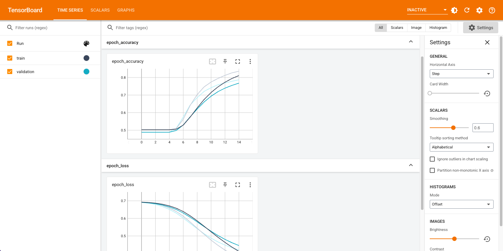
使用此方法,模型達到約 78% 的驗證準確度 (請注意,模型過度擬合,因為訓練準確度較高)。
您可以查看模型摘要,以進一步瞭解模型的每一層。
model.summary()
Model: "sequential"
_________________________________________________________________
 Layer (type)                Output Shape              Param #
=================================================================
 text_vectorization (TextVe  (None, 100)               0
 ctorization)

 embedding (Embedding)       (None, 100, 16)           160000

 global_average_pooling1d (  (None, 16)                0
 GlobalAveragePooling1D)

 dense (Dense)               (None, 16)                272

 dense_1 (Dense)             (None, 1)                 17

=================================================================
Total params: 160289 (626.13 KB)
Trainable params: 160289 (626.13 KB)
Non-trainable params: 0 (0.00 Byte)
_________________________________________________________________
在 TensorBoard 中視覺化模型指標。
#docs_infra: no_execute
%load_ext tensorboard
%tensorboard --logdir logs
擷取訓練過的詞嵌入並儲存到磁碟
接下來,擷取在訓練期間學習到的詞嵌入。嵌入是模型中嵌入層的權重。權重矩陣的形狀為 (vocab_size, embedding_dimension)。
使用 get_layer() 和 get_weights() 從模型取得權重。get_vocabulary() 函式提供詞彙表,以建構每行一個權杖的中繼資料檔案。
weights = model.get_layer('embedding').get_weights()[0]
vocab = vectorize_layer.get_vocabulary()
將權重寫入磁碟。若要使用 Embedding Projector,您將上傳兩個以 Tab 分隔格式的檔案:向量檔案 (包含嵌入) 和中繼資料檔案 (包含字詞)。
out_v = io.open('vectors.tsv', 'w', encoding='utf-8')
out_m = io.open('metadata.tsv', 'w', encoding='utf-8')

for index, word in enumerate(vocab):
  if index == 0:
    continue  # skip 0, it's padding.
  vec = weights[index]
  out_v.write('\t'.join([str(x) for x in vec]) + "\n")
  out_m.write(word + "\n")
out_v.close()
out_m.close()
如果您在 Colaboratory 中執行本教學課程,可以使用以下程式碼片段將這些檔案下載到您的本機 (或使用檔案瀏覽器,「檢視」->「目錄」->「檔案瀏覽器」)。
try:
  from google.colab import files
  files.download('vectors.tsv')
  files.download('metadata.tsv')
except Exception:
  pass
視覺化嵌入
若要視覺化嵌入,請將其上傳至 Embedding Projector。
開啟 Embedding Projector (這也可以在當地的 TensorBoard 執行個體中執行)。
按一下「載入資料」。
上傳您在上方建立的兩個檔案:
vecs.tsv和meta.tsv。
您訓練的嵌入現在將會顯示。您可以搜尋字詞以尋找最接近的鄰近字詞。例如,嘗試搜尋「beautiful」。您可能會看到「wonderful」等鄰近字詞。
後續步驟
本教學課程已示範如何在小型資料集上從頭開始訓練和視覺化詞嵌入。
若要使用 Word2Vec 演算法訓練詞嵌入,請嘗試 Word2Vec 教學課程。
如要進一步瞭解進階文字處理,請閱讀 Transformer 模型以瞭解語言。