
|
|
|
 在 GitHub 上檢視原始碼 在 GitHub 上檢視原始碼
|
|
|
本教學課程示範如何使用 TensorFlow Model Garden 微調雙向編碼器轉換器 (BERT) (Devlin et al., 2018) 模型。
您也可以在 TensorFlow Hub (TF Hub) 上找到本教學課程中使用的預先訓練 BERT 模型。如需瞭解如何使用 TF Hub 模型的具體範例,請參閱「使用 BERT 解決 Glue 任務」教學課程。如果您只是想微調模型,TF Hub 教學課程會是不錯的起點。
另一方面,如果您對更深入的自訂設定感興趣,請按照本教學課程操作。本教學課程說明如何手動完成許多操作,因此您可以學習如何自訂工作流程,從資料預先處理到模型訓練、匯出和儲存。
設定
安裝 pip 套件
首先安裝 TensorFlow Text 和 Model Garden pip 套件。
tf-models-official是 TensorFlow Model Garden 套件。請注意,其中可能未包含tensorflow_modelsGitHub 存放區中的最新變更。如要包含最新變更,您可以安裝tf-models-nightly,這是每日自動建立的 Model Garden 每夜版套件。- pip 將自動安裝所有模型和依附元件。
pip install -q opencv-python
pip install -q -U "tensorflow-text==2.11.*"
pip install -q tf-models-official
匯入程式庫
import os

import numpy as np
import matplotlib.pyplot as plt

import tensorflow as tf
import tensorflow_models as tfm
import tensorflow_hub as hub
import tensorflow_datasets as tfds
tfds.disable_progress_bar()
2024-02-07 12:13:37.890233: E external/local_xla/xla/stream_executor/cuda/cuda_dnn.cc:9261] Unable to register cuDNN factory: Attempting to register factory for plugin cuDNN when one has already been registered
2024-02-07 12:13:37.890282: E external/local_xla/xla/stream_executor/cuda/cuda_fft.cc:607] Unable to register cuFFT factory: Attempting to register factory for plugin cuFFT when one has already been registered
2024-02-07 12:13:37.891884: E external/local_xla/xla/stream_executor/cuda/cuda_blas.cc:1515] Unable to register cuBLAS factory: Attempting to register factory for plugin cuBLAS when one has already been registered
資源
以下目錄包含本教學課程中使用的 BERT 模型設定、詞彙表和預先訓練檢查點
gs_folder_bert = "gs://cloud-tpu-checkpoints/bert/v3/uncased_L-12_H-768_A-12"
tf.io.gfile.listdir(gs_folder_bert)
['bert_config.json',
 'bert_model.ckpt.data-00000-of-00001',
 'bert_model.ckpt.index',
 'vocab.txt']
載入並預先處理資料集
本範例使用來自 TensorFlow Datasets (TFDS) 的 GLUE (一般語言理解評估) MRPC (Microsoft Research Paraphrase Corpus) 資料集。
這個資料集並未設定為可以直接饋送至 BERT 模型。以下章節將處理必要的預先處理。
從 TensorFlow Datasets 取得資料集
GLUE MRPC (Dolan 和 Brockett,2005) 資料集是從線上新聞來源自動擷取的句子配對語料庫,並包含人工註解,說明配對中的句子是否在語意上等效。它具有下列屬性
- 標籤數量:2
- 訓練資料集大小:3668
- 評估資料集大小:408
- 訓練和評估資料集的最大序列長度:128
從載入 TFDS 的 MRPC 資料集開始
batch_size=32
glue, info = tfds.load('glue/mrpc',
                       with_info=True,
                       batch_size=32)
glue
{'train': <_PrefetchDataset element_spec={'idx': TensorSpec(shape=(None,), dtype=tf.int32, name=None), 'label': TensorSpec(shape=(None,), dtype=tf.int64, name=None), 'sentence1': TensorSpec(shape=(None,), dtype=tf.string, name=None), 'sentence2': TensorSpec(shape=(None,), dtype=tf.string, name=None)}>,
 'validation': <_PrefetchDataset element_spec={'idx': TensorSpec(shape=(None,), dtype=tf.int32, name=None), 'label': TensorSpec(shape=(None,), dtype=tf.int64, name=None), 'sentence1': TensorSpec(shape=(None,), dtype=tf.string, name=None), 'sentence2': TensorSpec(shape=(None,), dtype=tf.string, name=None)}>,
 'test': <_PrefetchDataset element_spec={'idx': TensorSpec(shape=(None,), dtype=tf.int32, name=None), 'label': TensorSpec(shape=(None,), dtype=tf.int64, name=None), 'sentence1': TensorSpec(shape=(None,), dtype=tf.string, name=None), 'sentence2': TensorSpec(shape=(None,), dtype=tf.string, name=None)}>}
info 物件說明資料集及其特徵
info.features
FeaturesDict({
    'idx': int32,
    'label': ClassLabel(shape=(), dtype=int64, num_classes=2),
    'sentence1': Text(shape=(), dtype=string),
    'sentence2': Text(shape=(), dtype=string),
})
兩個類別為
info.features['label'].names
['not_equivalent', 'equivalent']
以下是訓練集中的一個範例
example_batch = next(iter(glue['train']))

for key, value in example_batch.items():
  print(f"{key:9s}: {value[0].numpy()}")
idx      : 1680
label    : 0
sentence1: b'The identical rovers will act as robotic geologists , searching for evidence of past water .'
sentence2: b'The rovers act as robotic geologists , moving on six wheels .'
2024-02-07 12:13:45.153482: W tensorflow/core/kernels/data/cache_dataset_ops.cc:858] The calling iterator did not fully read the dataset being cached. In order to avoid unexpected truncation of the dataset, the partially cached contents of the dataset  will be discarded. This can happen if you have an input pipeline similar to `dataset.cache().take(k).repeat()`. You should use `dataset.take(k).cache().repeat()` instead.
預先處理資料
GLUE MRPC 資料集中的鍵 "sentence1" 和 "sentence2" 包含每個範例的兩個輸入句子。
由於 Model Garden 的 BERT 模型不接受原始文字做為輸入,因此首先需要完成兩件事
- 文字需要經過「符號化」(分割成字詞片段) 並轉換為「索引」。
- 接著,「索引」需要封裝成模型預期的格式。
BERT 符號器
如要微調 Model Garden 的預先訓練語言模型 (例如 BERT),您需要確保使用的符號化、詞彙表和索引對應與訓練期間使用的完全相同。
以下程式碼使用 Model Garden 的 tfm.nlp.layers.FastWordpieceBertTokenizer 層重建基礎模型使用的符號器
tokenizer = tfm.nlp.layers.FastWordpieceBertTokenizer(
    vocab_file=os.path.join(gs_folder_bert, "vocab.txt"),
    lower_case=True)
我們來符號化測試句子
tokens = tokenizer(tf.constant(["Hello TensorFlow!"]))
tokens
<tf.RaggedTensor [[[7592], [23435, 12314], [999]]]>
在「子字組符號化」和「使用 TensorFlow Text 進行符號化」指南中瞭解符號化程序的詳細資訊。
封裝輸入
TensorFlow Model Garden 的 BERT 模型不只接受符號化的字串做為輸入。它也預期這些字串會封裝成特定格式。tfm.nlp.layers.BertPackInputs 層可以處理從「符號化句子清單」到 Model Garden 的 BERT 模型預期輸入格式的轉換。
tfm.nlp.layers.BertPackInputs 會封裝串連在一起的兩個輸入句子 (MRCP 資料集中每個範例)。此輸入預期會以 [CLS]「這是一個分類問題」符號開頭,且每個句子應以 [SEP]「分隔符號」符號結尾。
因此,tfm.nlp.layers.BertPackInputs 層的建構函式會將 tokenizer 的特殊符號做為引數。它也需要知道符號器的特殊符號索引。
special = tokenizer.get_special_tokens_dict()
special
{'vocab_size': 30522,
 'start_of_sequence_id': 101,
 'end_of_segment_id': 102,
 'padding_id': 0,
 'mask_id': 103}
max_seq_length = 128

packer = tfm.nlp.layers.BertPackInputs(
    seq_length=max_seq_length,
    special_tokens_dict = tokenizer.get_special_tokens_dict())
packer 接受符號化句子清單做為輸入。例如
sentences1 = ["hello tensorflow"]
tok1 = tokenizer(sentences1)
tok1
<tf.RaggedTensor [[[7592], [23435, 12314]]]>
sentences2 = ["goodbye tensorflow"]
tok2 = tokenizer(sentences2)
tok2
<tf.RaggedTensor [[[9119], [23435, 12314]]]>
接著,它會傳回包含三個輸出的字典
input_word_ids:封裝在一起的符號化句子。input_mask:遮罩,指出其他輸出中哪些位置有效。input_type_ids:指出每個符號所屬的句子。
packed = packer([tok1, tok2])

for key, tensor in packed.items():
  print(f"{key:15s}: {tensor[:, :12]}")
input_word_ids : [[  101  7592 23435 12314   102  9119 23435 12314   102     0     0     0]]
input_mask     : [[1 1 1 1 1 1 1 1 1 0 0 0]]
input_type_ids : [[0 0 0 0 0 1 1 1 1 0 0 0]]
整合所有項目
將這兩個部分合併為可附加至模型的 keras.layers.Layer
class BertInputProcessor(tf.keras.layers.Layer):
  def __init__(self, tokenizer, packer):
    super().__init__()
    self.tokenizer = tokenizer
    self.packer = packer

  def call(self, inputs):
    tok1 = self.tokenizer(inputs['sentence1'])
    tok2 = self.tokenizer(inputs['sentence2'])

    packed = self.packer([tok1, tok2])

    if 'label' in inputs:
      return packed, inputs['label']
    else:
      return packed
但現在只需使用 Dataset.map 將其套用至資料集,因為您從 TFDS 載入的資料集是 tf.data.Dataset 物件
bert_inputs_processor = BertInputProcessor(tokenizer, packer)
glue_train = glue['train'].map(bert_inputs_processor).prefetch(1)
以下是已處理資料集的範例批次
example_inputs, example_labels = next(iter(glue_train))
2024-02-07 12:13:49.744645: W tensorflow/core/kernels/data/cache_dataset_ops.cc:858] The calling iterator did not fully read the dataset being cached. In order to avoid unexpected truncation of the dataset, the partially cached contents of the dataset will be discarded. This can happen if you have an input pipeline similar to `dataset.cache().take(k).repeat()`. You should use `dataset.take(k).cache().repeat()` instead.
example_inputs
{'input_word_ids': <tf.Tensor: shape=(32, 128), dtype=int32, numpy=
 array([[ 101, 1996, 7235, ...,    0,    0,    0],
        [ 101, 2625, 2084, ...,    0,    0,    0],
        [ 101, 6804, 1011, ...,    0,    0,    0],
        ...,
        [ 101, 2021, 2049, ...,    0,    0,    0],
        [ 101, 2274, 2062, ...,    0,    0,    0],
        [ 101, 2043, 1037, ...,    0,    0,    0]], dtype=int32)>,
 'input_mask': <tf.Tensor: shape=(32, 128), dtype=int32, numpy=
 array([[1, 1, 1, ..., 0, 0, 0],
        [1, 1, 1, ..., 0, 0, 0],
        [1, 1, 1, ..., 0, 0, 0],
        ...,
        [1, 1, 1, ..., 0, 0, 0],
        [1, 1, 1, ..., 0, 0, 0],
        [1, 1, 1, ..., 0, 0, 0]], dtype=int32)>,
 'input_type_ids': <tf.Tensor: shape=(32, 128), dtype=int32, numpy=
 array([[0, 0, 0, ..., 0, 0, 0],
        [0, 0, 0, ..., 0, 0, 0],
        [0, 0, 0, ..., 0, 0, 0],
        ...,
        [0, 0, 0, ..., 0, 0, 0],
        [0, 0, 0, ..., 0, 0, 0],
        [0, 0, 0, ..., 0, 0, 0]], dtype=int32)>}
example_labels
<tf.Tensor: shape=(32,), dtype=int64, numpy=
array([0, 0, 1, 1, 0, 0, 1, 1, 1, 1, 1, 1, 0, 1, 1, 0, 1, 1, 1, 0, 1, 1,
       1, 1, 1, 1, 1, 0, 0, 1, 0, 1])>
for key, value in example_inputs.items():
  print(f'{key:15s} shape: {value.shape}')

print(f'{"labels":15s} shape: {example_labels.shape}')
input_word_ids  shape: (32, 128)
input_mask      shape: (32, 128)
input_type_ids  shape: (32, 128)
labels          shape: (32,)
input_word_ids 包含符號 ID
plt.pcolormesh(example_inputs['input_word_ids'])
<matplotlib.collections.QuadMesh at 0x7f0f10480250>
遮罩可讓模型清楚區分內容和填補。遮罩的形狀與 input_word_ids 相同,且在 input_word_ids 不是填補的任何位置都包含 1。
plt.pcolormesh(example_inputs['input_mask'])
<matplotlib.collections.QuadMesh at 0x7f0f500ce670>
「輸入類型」也具有相同的形狀,但在未填補的區域內,包含 0 或 1,指出符號是哪個句子的一部分。
plt.pcolormesh(example_inputs['input_type_ids'])
<matplotlib.collections.QuadMesh at 0x7f0f201d4700>
將相同的預先處理套用至 GLUE MRPC 資料集的驗證和測試子集
glue_validation = glue['validation'].map(bert_inputs_processor).prefetch(1)
glue_test = glue['test'].map(bert_inputs_processor).prefetch(1)
建構、訓練及匯出模型
現在您已將資料格式化為預期格式,可以開始建構和訓練模型。
建構模型
第一步是下載預先訓練 BERT 模型的設定檔—config_dict
import json

bert_config_file = os.path.join(gs_folder_bert, "bert_config.json")
config_dict = json.loads(tf.io.gfile.GFile(bert_config_file).read())
config_dict
{'attention_probs_dropout_prob': 0.1,
 'hidden_act': 'gelu',
 'hidden_dropout_prob': 0.1,
 'hidden_size': 768,
 'initializer_range': 0.02,
 'intermediate_size': 3072,
 'max_position_embeddings': 512,
 'num_attention_heads': 12,
 'num_hidden_layers': 12,
 'type_vocab_size': 2,
 'vocab_size': 30522}
encoder_config = tfm.nlp.encoders.EncoderConfig({
    'type':'bert',
    'bert': config_dict
})
bert_encoder = tfm.nlp.encoders.build_encoder(encoder_config)
bert_encoder
<official.nlp.modeling.networks.bert_encoder.BertEncoder at 0x7f0f103d16d0>
設定檔定義 Model Garden 的核心 BERT 模型,這是一個 Keras 模型,可從最大序列長度 max_seq_length 的輸入預測 num_classes 的輸出。
bert_classifier = tfm.nlp.models.BertClassifier(network=bert_encoder, num_classes=2)
在來自訓練集的 10 個範例的測試批次資料上執行。輸出是兩個類別的 logits
bert_classifier(
    example_inputs, training=True).numpy()[:10]
array([[ 0.08335936,  1.1473498 ],
       [ 1.3190541 ,  1.3408866 ],
       [ 0.19908446,  0.7913456 ],
       [ 0.48186374,  1.2114024 ],
       [ 0.9708527 ,  0.7837988 ],
       [ 0.25541633,  0.76591694],
       [ 1.3683597 ,  1.0795705 ],
       [ 0.11288509,  1.1301354 ],
       [-0.02536219,  0.4678782 ],
       [ 0.9831672 ,  0.538211  ]], dtype=float32)
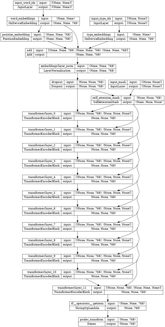
上方分類器中心的 TransformerEncoder 「就是」bert_encoder。
如果您檢查編碼器,會注意到連接到這三個相同輸入的 Transformer 層堆疊
tf.keras.utils.plot_model(bert_encoder, show_shapes=True, dpi=48)
還原編碼器權重
建構時,編碼器會隨機初始化。從檢查點還原編碼器的權重
checkpoint = tf.train.Checkpoint(encoder=bert_encoder)
checkpoint.read(
    os.path.join(gs_folder_bert, 'bert_model.ckpt')).assert_consumed()
<tensorflow.python.checkpoint.checkpoint.CheckpointLoadStatus at 0x7f105f713cd0>
設定最佳化工具
BERT 通常使用具有權重衰減的 Adam 最佳化工具—AdamW (AdamW (tf.keras.optimizers.experimental.AdamW))。它也採用學習率排程,先從 0 開始預熱,然後衰減至 0
# Set up epochs and steps
epochs = 5
batch_size = 32
eval_batch_size = 32

train_data_size = info.splits['train'].num_examples
steps_per_epoch = int(train_data_size / batch_size)
num_train_steps = steps_per_epoch * epochs
warmup_steps = int(0.1 * num_train_steps)
initial_learning_rate=2e-5
從 initial_learning_rate 到零的線性衰減,超過 num_train_steps。
linear_decay = tf.keras.optimizers.schedules.PolynomialDecay(
    initial_learning_rate=initial_learning_rate,
    end_learning_rate=0,
    decay_steps=num_train_steps)
在 warmup_steps 內預熱至該值
warmup_schedule = tfm.optimization.lr_schedule.LinearWarmup(
    warmup_learning_rate = 0,
    after_warmup_lr_sched = linear_decay,
    warmup_steps = warmup_steps
)
整體排程如下所示
x = tf.linspace(0, num_train_steps, 1001)
y = [warmup_schedule(xi) for xi in x]
plt.plot(x,y)
plt.xlabel('Train step')
plt.ylabel('Learning rate')
Text(0, 0.5, 'Learning rate')
使用 tf.keras.optimizers.experimental.AdamW 具現化具有該排程的最佳化工具
optimizer = tf.keras.optimizers.experimental.Adam(
    learning_rate = warmup_schedule)
訓練模型
將指標設為準確度,並將損失設為稀疏類別交叉熵。接著,編譯和訓練 BERT 分類器
metrics = [tf.keras.metrics.SparseCategoricalAccuracy('accuracy', dtype=tf.float32)]
loss = tf.keras.losses.SparseCategoricalCrossentropy(from_logits=True)

bert_classifier.compile(
    optimizer=optimizer,
    loss=loss,
    metrics=metrics)
bert_classifier.evaluate(glue_validation)
13/13 [==============================] - 6s 255ms/step - loss: 1.1962 - accuracy: 0.3162
[1.1962156295776367, 0.31617647409439087]
bert_classifier.fit(
      glue_train,
      validation_data=(glue_validation),
      batch_size=32,
      epochs=epochs)
Epoch 1/5
WARNING: All log messages before absl::InitializeLog() is called are written to STDERR
I0000 00:00:1707308071.926522   10692 device_compiler.h:186] Compiled cluster using XLA!  This line is logged at most once for the lifetime of the process.
115/115 [==============================] - 131s 858ms/step - loss: 0.7210 - accuracy: 0.6191 - val_loss: 0.5249 - val_accuracy: 0.7426
Epoch 2/5
115/115 [==============================] - 101s 875ms/step - loss: 0.4744 - accuracy: 0.7751 - val_loss: 0.4766 - val_accuracy: 0.8064
Epoch 3/5
115/115 [==============================] - 101s 877ms/step - loss: 0.3204 - accuracy: 0.8642 - val_loss: 0.4100 - val_accuracy: 0.8333
Epoch 4/5
115/115 [==============================] - 101s 878ms/step - loss: 0.2006 - accuracy: 0.9278 - val_loss: 0.4783 - val_accuracy: 0.8358
Epoch 5/5
115/115 [==============================] - 101s 879ms/step - loss: 0.1323 - accuracy: 0.9577 - val_loss: 0.4668 - val_accuracy: 0.8382
<keras.src.callbacks.History at 0x7f105f702250>
現在在自訂範例上執行微調模型,看看它是否運作。
從編碼一些句子配對開始
my_examples = {
        'sentence1':[
            'The rain in Spain falls mainly on the plain.',
            'Look I fine tuned BERT.'],
        'sentence2':[
            'It mostly rains on the flat lands of Spain.',
            'Is it working? This does not match.']
    }
模型應針對第一個範例回報類別 1「符合」,針對第二個範例回報類別 0「不符合」
ex_packed = bert_inputs_processor(my_examples)
my_logits = bert_classifier(ex_packed, training=False)

result_cls_ids = tf.argmax(my_logits)
result_cls_ids
<tf.Tensor: shape=(2,), dtype=int64, numpy=array([1, 0])>
tf.gather(tf.constant(info.features['label'].names), result_cls_ids)
<tf.Tensor: shape=(2,), dtype=string, numpy=array([b'equivalent', b'not_equivalent'], dtype=object)>
匯出模型
訓練模型的目標通常是「使用」它來執行建立它的 Python 流程之外的作業。您可以使用 tf.saved_model 匯出模型來完成此操作。(如要瞭解詳情,請參閱「使用 SavedModel 格式」指南和「使用分配策略儲存及載入模型」教學課程。)
首先,建構包裝類別以匯出模型。這個包裝類別會執行兩項操作
- 首先,它將
bert_inputs_processor和bert_classifier一起封裝到單一tf.Module中,以便您可以匯出所有功能。 - 其次,它定義一個
tf.function,用於實作模型的端對端執行。
設定 tf.function 的 input_signature 引數可讓您為 tf.function 定義固定簽名。這可能比預設的自動重新追蹤行為更令人感到驚訝。
class ExportModel(tf.Module):
  def __init__(self, input_processor, classifier):
    self.input_processor = input_processor
    self.classifier = classifier

  @tf.function(input_signature=[{
      'sentence1': tf.TensorSpec(shape=[None], dtype=tf.string),
      'sentence2': tf.TensorSpec(shape=[None], dtype=tf.string)}])
  def __call__(self, inputs):
    packed = self.input_processor(inputs)
    logits =  self.classifier(packed, training=False)
    result_cls_ids = tf.argmax(logits)
    return {
        'logits': logits,
        'class_id': result_cls_ids,
        'class': tf.gather(
            tf.constant(info.features['label'].names),
            result_cls_ids)
    }
建立這個匯出模型的執行個體並儲存
export_model = ExportModel(bert_inputs_processor, bert_classifier)
import tempfile
export_dir=tempfile.mkdtemp(suffix='_saved_model')
tf.saved_model.save(export_model, export_dir=export_dir,
                    signatures={'serving_default': export_model.__call__})
INFO:tensorflow:Assets written to: /tmpfs/tmp/tmpxj846i17_saved_model/assets
INFO:tensorflow:Assets written to: /tmpfs/tmp/tmpxj846i17_saved_model/assets
重新載入模型,並將結果與原始模型進行比較
original_logits = export_model(my_examples)['logits']
reloaded = tf.saved_model.load(export_dir)
reloaded_logits = reloaded(my_examples)['logits']
# The results are identical:
print(original_logits.numpy())
print()
print(reloaded_logits.numpy())
[[-2.7769644  2.3126464]
 [ 1.4339567 -1.1664971]]

[[-2.7769644  2.3126464]
 [ 1.4339567 -1.1664971]]
print(np.mean(abs(original_logits - reloaded_logits)))
0.0
恭喜!您已使用 tensorflow_models 建構 BERT 分類器、訓練並匯出它以供日後使用。
選用:TF Hub 上的 BERT
您可以從 TF Hub 取得現成的 BERT 模型。有許多版本及其輸入預先處理器可供使用。
本範例使用來自 TF Hub 的小型 BERT 版本,該版本使用英文 Wikipedia 和 BooksCorpus 資料集進行預先訓練,類似於原始實作 (Turc et al., 2019)。
從匯入 TF Hub 開始
import tensorflow_hub as hub
從 TF Hub 選取輸入預先處理器和模型,並將它們包裝為 hub.KerasLayer 層
# Always make sure you use the right preprocessor.
hub_preprocessor = hub.KerasLayer(
    "https://tfhub.dev/tensorflow/bert_en_uncased_preprocess/3")

# This is a really small BERT.
hub_encoder = hub.KerasLayer(f"https://tfhub.dev/tensorflow/small_bert/bert_en_uncased_L-2_H-128_A-2/2",
                             trainable=True)

print(f"The Hub encoder has {len(hub_encoder.trainable_variables)} trainable variables")
The Hub encoder has 39 trainable variables
在批次資料上測試執行預先處理器
hub_inputs = hub_preprocessor(['Hello TensorFlow!'])
{key: value[0, :10].numpy() for key, value in hub_inputs.items()}
{'input_type_ids': array([0, 0, 0, 0, 0, 0, 0, 0, 0, 0], dtype=int32),
 'input_word_ids': array([  101,  7592, 23435, 12314,   999,   102,     0,     0,     0,
            0], dtype=int32),
 'input_mask': array([1, 1, 1, 1, 1, 1, 0, 0, 0, 0], dtype=int32)}
result = hub_encoder(
    inputs=hub_inputs,
    training=False,
)

print("Pooled output shape:", result['pooled_output'].shape)
print("Sequence output shape:", result['sequence_output'].shape)
Pooled output shape: (1, 128)
Sequence output shape: (1, 128, 128)
此時,您可以輕鬆自行新增分類標頭。
Model Garden tfm.nlp.models.BertClassifier 類別也可以在 TF Hub 編碼器上建構分類器
hub_classifier = tfm.nlp.models.BertClassifier(
    bert_encoder,
    num_classes=2,
    dropout_rate=0.1,
    initializer=tf.keras.initializers.TruncatedNormal(
        stddev=0.02))
從 TF Hub 載入此模型的缺點之一是內部 Keras 層的結構未還原。這使得檢查或修改模型更加困難。
BERT 編碼器模型—hub_classifier—現在是單一層。
如需此方法的具體範例,請參閱「使用 BERT 解決 Glue 任務」。
選用:最佳化工具 config
tensorflow_models 套件定義可序列化的 config 類別,用於說明如何建構即時物件。在本教學課程稍早的部分,您已手動建構最佳化工具。
以下設定說明由 optimizer_factory.OptimizerFactory 建構的 (幾乎) 相同的最佳化工具
optimization_config = tfm.optimization.OptimizationConfig(
    optimizer=tfm.optimization.OptimizerConfig(
        type = "adam"),
    learning_rate = tfm.optimization.LrConfig(
        type='polynomial',
        polynomial=tfm.optimization.PolynomialLrConfig(
            initial_learning_rate=2e-5,
            end_learning_rate=0.0,
            decay_steps=num_train_steps)),
    warmup = tfm.optimization.WarmupConfig(
        type='linear',
        linear=tfm.optimization.LinearWarmupConfig(warmup_steps=warmup_steps)
    ))


fac = tfm.optimization.optimizer_factory.OptimizerFactory(optimization_config)
lr = fac.build_learning_rate()
optimizer = fac.build_optimizer(lr=lr)
x = tf.linspace(0, num_train_steps, 1001).numpy()
y = [lr(xi) for xi in x]
plt.plot(x,y)
plt.xlabel('Train step')
plt.ylabel('Learning rate')
Text(0, 0.5, 'Learning rate')
使用 config 物件的優點是它們不包含任何複雜的 TensorFlow 物件,而且可以輕鬆序列化為 JSON 並重建。以下是上述 tfm.optimization.OptimizationConfig 的 JSON
optimization_config = optimization_config.as_dict()
optimization_config
{'optimizer': {'type': 'adam',
  'adam': {'clipnorm': None,
   'clipvalue': None,
   'global_clipnorm': None,
   'name': 'Adam',
   'beta_1': 0.9,
   'beta_2': 0.999,
   'epsilon': 1e-07,
   'amsgrad': False} },
 'ema': None,
 'learning_rate': {'type': 'polynomial',
  'polynomial': {'name': 'PolynomialDecay',
   'initial_learning_rate': 2e-05,
   'decay_steps': 570,
   'end_learning_rate': 0.0,
   'power': 1.0,
   'cycle': False,
   'offset': 0} },
 'warmup': {'type': 'linear',
  'linear': {'name': 'linear', 'warmup_learning_rate': 0, 'warmup_steps': 57} } }
tfm.optimization.optimizer_factory.OptimizerFactory 可以同樣輕鬆地從 JSON 字典建構最佳化工具
fac = tfm.optimization.optimizer_factory.OptimizerFactory(
    tfm.optimization.OptimizationConfig(optimization_config))
lr = fac.build_learning_rate()
optimizer = fac.build_optimizer(lr=lr)