
|
|
|
 在 GitHub 上檢視原始碼 在 GitHub 上檢視原始碼
|
|
|
總覽
這個筆記本使用評論文字將電影評論分類為正面或負面。這是二元分類的範例,二元分類是一種重要且廣泛適用的機器學習問題。
我們將在本筆記本中示範如何使用圖形正規化,方法是從給定的輸入建立圖形。當輸入不包含明確的圖形時,使用神經結構化學習 (NSL) 架構建構圖形正規化模型的一般步驟如下:
- 為輸入中的每個文字範例建立嵌入。這可以使用預先訓練的模型來完成,例如 word2vec、Swivel、BERT 等。
- 根據這些嵌入建立圖形,方法是使用相似度指標,例如「L2」距離、「餘弦」距離等。圖形中的節點對應於範例,而圖形中的邊緣對應於範例對之間的相似度。
- 從上述合成圖形和範例特徵產生訓練資料。產生的訓練資料除了原始節點特徵外,還會包含鄰近節點特徵。
- 使用 Keras 序列、功能或子類別 API 建立神經網路作為基礎模型。
- 使用 NSL 架構提供的 GraphRegularization 包裝函式類別包裝基礎模型,以建立新的圖形 Keras 模型。這個新模型將包含圖形正規化損失,作為其訓練目標中的正規化項。
- 訓練和評估圖形 Keras 模型。
需求條件
- 安裝神經結構化學習套件。
- 安裝 tensorflow-hub。
pip install --quiet neural-structured-learningpip install --quiet tensorflow-hub
依附元件和匯入
import matplotlib.pyplot as plt
import numpy as np

import neural_structured_learning as nsl

import tensorflow as tf
import tensorflow_hub as hub

# Resets notebook state
tf.keras.backend.clear_session()

print("Version: ", tf.__version__)
print("Eager mode: ", tf.executing_eagerly())
print("Hub version: ", hub.__version__)
print(
    "GPU is",
    "available" if tf.config.list_physical_devices("GPU") else "NOT AVAILABLE")
2022-12-14 12:19:13.551836: W tensorflow/compiler/xla/stream_executor/platform/default/dso_loader.cc:64] Could not load dynamic library 'libnvinfer.so.7'; dlerror: libnvinfer.so.7: cannot open shared object file: No such file or directory
2022-12-14 12:19:13.551949: W tensorflow/compiler/xla/stream_executor/platform/default/dso_loader.cc:64] Could not load dynamic library 'libnvinfer_plugin.so.7'; dlerror: libnvinfer_plugin.so.7: cannot open shared object file: No such file or directory
2022-12-14 12:19:13.551962: W tensorflow/compiler/tf2tensorrt/utils/py_utils.cc:38] TF-TRT Warning: Cannot dlopen some TensorRT libraries. If you would like to use Nvidia GPU with TensorRT, please make sure the missing libraries mentioned above are installed properly.
Version:  2.11.0
Eager mode:  True
Hub version:  0.12.0
GPU is NOT AVAILABLE
2022-12-14 12:19:14.770677: E tensorflow/compiler/xla/stream_executor/cuda/cuda_driver.cc:267] failed call to cuInit: CUDA_ERROR_NO_DEVICE: no CUDA-capable device is detected
IMDB 資料集
IMDB 資料集包含來自 網際網路電影資料庫的 50,000 則電影評論文字。這些評論分為 25,000 則訓練評論和 25,000 則測試評論。訓練和測試集是平衡的,表示它們包含數量相等的正面和負面評論。
在本教學課程中,我們將使用預先處理過的 IMDB 資料集版本。
下載預先處理過的 IMDB 資料集
IMDB 資料集隨 TensorFlow 一起封裝。它已經過預先處理,因此評論 (文字序列) 已轉換為整數序列,其中每個整數代表字典中的特定字詞。
以下程式碼會下載 IMDB 資料集 (或使用已下載的快取副本)
imdb = tf.keras.datasets.imdb
(pp_train_data, pp_train_labels), (pp_test_data, pp_test_labels) = (
    imdb.load_data(num_words=10000))
Downloading data from https://storage.googleapis.com/tensorflow/tf-keras-datasets/imdb.npz
17464789/17464789 [==============================] - 0s 0us/step
num_words=10000 引數會保留訓練資料中前 10,000 個最常出現的字詞。罕見字詞會被捨棄,以保持詞彙表大小可管理。
探索資料
讓我們花點時間瞭解資料的格式。資料集已預先處理:每個範例都是代表電影評論字詞的整數陣列。每個標籤都是 0 或 1 的整數值,其中 0 是負面評論,1 是正面評論。
print('Training entries: {}, labels: {}'.format(
    len(pp_train_data), len(pp_train_labels)))
training_samples_count = len(pp_train_data)
Training entries: 25000, labels: 25000
評論文字已轉換為整數,其中每個整數代表字典中的特定字詞。以下是第一則評論的外觀
print(pp_train_data[0])
[1, 14, 22, 16, 43, 530, 973, 1622, 1385, 65, 458, 4468, 66, 3941, 4, 173, 36, 256, 5, 25, 100, 43, 838, 112, 50, 670, 2, 9, 35, 480, 284, 5, 150, 4, 172, 112, 167, 2, 336, 385, 39, 4, 172, 4536, 1111, 17, 546, 38, 13, 447, 4, 192, 50, 16, 6, 147, 2025, 19, 14, 22, 4, 1920, 4613, 469, 4, 22, 71, 87, 12, 16, 43, 530, 38, 76, 15, 13, 1247, 4, 22, 17, 515, 17, 12, 16, 626, 18, 2, 5, 62, 386, 12, 8, 316, 8, 106, 5, 4, 2223, 5244, 16, 480, 66, 3785, 33, 4, 130, 12, 16, 38, 619, 5, 25, 124, 51, 36, 135, 48, 25, 1415, 33, 6, 22, 12, 215, 28, 77, 52, 5, 14, 407, 16, 82, 2, 8, 4, 107, 117, 5952, 15, 256, 4, 2, 7, 3766, 5, 723, 36, 71, 43, 530, 476, 26, 400, 317, 46, 7, 4, 2, 1029, 13, 104, 88, 4, 381, 15, 297, 98, 32, 2071, 56, 26, 141, 6, 194, 7486, 18, 4, 226, 22, 21, 134, 476, 26, 480, 5, 144, 30, 5535, 18, 51, 36, 28, 224, 92, 25, 104, 4, 226, 65, 16, 38, 1334, 88, 12, 16, 283, 5, 16, 4472, 113, 103, 32, 15, 16, 5345, 19, 178, 32]
電影評論的長度可能不同。以下程式碼顯示第一則和第二則評論中的字詞數。由於神經網路的輸入長度必須相同,因此我們稍後需要解決這個問題。
len(pp_train_data[0]), len(pp_train_data[1])
(218, 189)
將整數轉換回字詞
瞭解如何將整數轉換回對應的文字可能很有用。在這裡,我們將建立一個輔助函式來查詢包含整數到字串對應的字典物件
def build_reverse_word_index():
  # A dictionary mapping words to an integer index
  word_index = imdb.get_word_index()

  # The first indices are reserved
  word_index = {k: (v + 3) for k, v in word_index.items()}
  word_index['<PAD>'] = 0
  word_index['<START>'] = 1
  word_index['<UNK>'] = 2  # unknown
  word_index['<UNUSED>'] = 3
  return dict((value, key) for (key, value) in word_index.items())

reverse_word_index = build_reverse_word_index()

def decode_review(text):
  return ' '.join([reverse_word_index.get(i, '?') for i in text])
Downloading data from https://storage.googleapis.com/tensorflow/tf-keras-datasets/imdb_word_index.json
1641221/1641221 [==============================] - 0s 0us/step
現在我們可以利用 decode_review 函式顯示第一則評論的文字
decode_review(pp_train_data[0])
"<START> this film was just brilliant casting location scenery story direction everyone's really suited the part they played and you could just imagine being there robert <UNK> is an amazing actor and now the same being director <UNK> father came from the same scottish island as myself so i loved the fact there was a real connection with this film the witty remarks throughout the film were great it was just brilliant so much that i bought the film as soon as it was released for <UNK> and would recommend it to everyone to watch and the fly fishing was amazing really cried at the end it was so sad and you know what they say if you cry at a film it must have been good and this definitely was also <UNK> to the two little boy's that played the <UNK> of norman and paul they were just brilliant children are often left out of the <UNK> list i think because the stars that play them all grown up are such a big profile for the whole film but these children are amazing and should be praised for what they have done don't you think the whole story was so lovely because it was true and was someone's life after all that was shared with us all"
圖形建構
圖形建構涉及為文字範例建立嵌入,然後使用相似度函式比較嵌入。
在繼續之前,我們先建立一個目錄來儲存本教學課程建立的成品。
mkdir -p /tmp/imdb
建立範例嵌入
我們將使用預先訓練的 Swivel 嵌入,以 tf.train.Example 格式為輸入中的每個範例建立嵌入。我們將以 TFRecord 格式儲存產生的嵌入,以及代表每個範例 ID 的額外特徵。這很重要,稍後可讓我們將範例嵌入與圖形中的對應節點進行比對。
pretrained_embedding = 'https://tfhub.dev/google/tf2-preview/gnews-swivel-20dim/1'

hub_layer = hub.KerasLayer(
    pretrained_embedding, input_shape=[], dtype=tf.string, trainable=True)
WARNING:tensorflow:Please fix your imports. Module tensorflow.python.training.tracking.data_structures has been moved to tensorflow.python.trackable.data_structures. The old module will be deleted in version 2.11.
def _int64_feature(value):
  """Returns int64 tf.train.Feature."""
  return tf.train.Feature(int64_list=tf.train.Int64List(value=value.tolist()))


def _bytes_feature(value):
  """Returns bytes tf.train.Feature."""
  return tf.train.Feature(
      bytes_list=tf.train.BytesList(value=[value.encode('utf-8')]))


def _float_feature(value):
  """Returns float tf.train.Feature."""
  return tf.train.Feature(float_list=tf.train.FloatList(value=value.tolist()))


def create_embedding_example(word_vector, record_id):
  """Create tf.Example containing the sample's embedding and its ID."""

  text = decode_review(word_vector)

  # Shape = [batch_size,].
  sentence_embedding = hub_layer(tf.reshape(text, shape=[-1,]))

  # Flatten the sentence embedding back to 1-D.
  sentence_embedding = tf.reshape(sentence_embedding, shape=[-1])

  features = {
      'id': _bytes_feature(str(record_id)),
      'embedding': _float_feature(sentence_embedding.numpy())
  }
  return tf.train.Example(features=tf.train.Features(feature=features))


def create_embeddings(word_vectors, output_path, starting_record_id):
  record_id = int(starting_record_id)
  with tf.io.TFRecordWriter(output_path) as writer:
    for word_vector in word_vectors:
      example = create_embedding_example(word_vector, record_id)
      record_id = record_id + 1
      writer.write(example.SerializeToString())
  return record_id


# Persist TF.Example features containing embeddings for training data in
# TFRecord format.
create_embeddings(pp_train_data, '/tmp/imdb/embeddings.tfr', 0)
25000
建構圖形
現在我們有了範例嵌入,我們將使用它們來建構相似度圖形,也就是說,此圖形中的節點將對應於範例,而此圖形中的邊緣將對應於節點對之間的相似度。
神經結構化學習提供圖形建構程式庫,可根據範例嵌入建構圖形。它使用 餘弦相似度 作為相似度量值來比較嵌入,並在它們之間建立邊緣。它也允許我們指定相似度閾值,可用於從最終圖形中捨棄不相似的邊緣。在本範例中,使用 0.99 作為相似度閾值,並使用 12345 作為隨機種子,我們最終得到一個具有 429,415 個雙向邊緣的圖形。在這裡,我們使用圖形建構器的 局部敏感雜湊 (LSH) 支援來加速圖形建構。如需使用圖形建構器的 LSH 支援的詳細資訊,請參閱 build_graph_from_config API 文件。
graph_builder_config = nsl.configs.GraphBuilderConfig(
    similarity_threshold=0.99, lsh_splits=32, lsh_rounds=15, random_seed=12345)
nsl.tools.build_graph_from_config(['/tmp/imdb/embeddings.tfr'],
                                  '/tmp/imdb/graph_99.tsv',
                                  graph_builder_config)
每個雙向邊緣都由輸出 TSV 檔案中的兩個有向邊緣表示,因此該檔案包含 429,415 * 2 = 858,830 行
wc -l /tmp/imdb/graph_99.tsv
858830 /tmp/imdb/graph_99.tsv
範例特徵
我們使用 tf.train.Example 格式建立問題的範例特徵,並將它們以 TFRecord 格式保存。每個範例將包含以下三個特徵
- id:範例的節點 ID。
- words:包含字詞 ID 的 int64 清單。
- label:識別評論目標類別的單例 int64。
def create_example(word_vector, label, record_id):
  """Create tf.Example containing the sample's word vector, label, and ID."""
  features = {
      'id': _bytes_feature(str(record_id)),
      'words': _int64_feature(np.asarray(word_vector)),
      'label': _int64_feature(np.asarray([label])),
  }
  return tf.train.Example(features=tf.train.Features(feature=features))

def create_records(word_vectors, labels, record_path, starting_record_id):
  record_id = int(starting_record_id)
  with tf.io.TFRecordWriter(record_path) as writer:
    for word_vector, label in zip(word_vectors, labels):
      example = create_example(word_vector, label, record_id)
      record_id = record_id + 1
      writer.write(example.SerializeToString())
  return record_id

# Persist TF.Example features (word vectors and labels) for training and test
# data in TFRecord format.
next_record_id = create_records(pp_train_data, pp_train_labels,
                                '/tmp/imdb/train_data.tfr', 0)
create_records(pp_test_data, pp_test_labels, '/tmp/imdb/test_data.tfr',
               next_record_id)
50000
使用圖形鄰近節點擴增訓練資料
由於我們有範例特徵和合成圖形,因此我們可以產生用於神經結構化學習的擴增訓練資料。NSL 架構提供了一個程式庫,可結合圖形和範例特徵,以產生用於圖形正規化的最終訓練資料。產生的訓練資料將包含原始範例特徵以及其對應鄰近節點的特徵。
在本教學課程中,我們考慮無向邊緣,並對每個範例使用最多 3 個鄰近節點,以使用圖形鄰近節點擴增訓練資料。
nsl.tools.pack_nbrs(
    '/tmp/imdb/train_data.tfr',
    '',
    '/tmp/imdb/graph_99.tsv',
    '/tmp/imdb/nsl_train_data.tfr',
    add_undirected_edges=True,
    max_nbrs=3)
基礎模型
我們現在準備好在沒有圖形正規化的情況下建構基礎模型。為了建構此模型,我們可以使用在建構圖形時使用的嵌入,也可以與分類任務一起聯合學習新的嵌入。就本筆記本而言,我們將採用後者。
全域變數
NBR_FEATURE_PREFIX = 'NL_nbr_'
NBR_WEIGHT_SUFFIX = '_weight'
超參數
我們將使用 HParams 的執行個體來包含用於訓練和評估的各種超參數和常數。我們在下面簡要說明其中每一個
num_classes:有 2 個類別 -- 正面和負面。
max_seq_length:這是本範例中從每部電影評論中考量的最大字詞數。
vocab_size:這是本範例中考量的詞彙表大小。
distance_type:這是用於使用其鄰近節點正規化範例的距離度量。
graph_regularization_multiplier:這會控制圖形正規化項在整體損失函數中的相對權重。
num_neighbors:用於圖形正規化的鄰近節點數。此值必須小於或等於在叫用
nsl.tools.pack_nbrs時使用的max_nbrs引數。num_fc_units:神經網路中全連線層的單元數。
train_epochs:訓練週期數。
batch_size:用於訓練和評估的批次大小。
eval_steps:在認為評估完成之前要處理的批次數。如果設定為
None,則會評估測試集中的所有執行個體。
class HParams(object):
  """Hyperparameters used for training."""
  def __init__(self):
    ### dataset parameters
    self.num_classes = 2
    self.max_seq_length = 256
    self.vocab_size = 10000
    ### neural graph learning parameters
    self.distance_type = nsl.configs.DistanceType.L2
    self.graph_regularization_multiplier = 0.1
    self.num_neighbors = 2
    ### model architecture
    self.num_embedding_dims = 16
    self.num_lstm_dims = 64
    self.num_fc_units = 64
    ### training parameters
    self.train_epochs = 10
    self.batch_size = 128
    ### eval parameters
    self.eval_steps = None  # All instances in the test set are evaluated.

HPARAMS = HParams()
準備資料
評論 (整數陣列) 必須先轉換為張量,才能饋送至神經網路。此轉換可以透過幾種方式完成
將陣列轉換為
0和1的向量,以指示字詞出現次數,類似於單熱編碼。例如,序列[3, 5]會變成一個10000維向量,除了索引3和5(為 1) 之外,其餘皆為零。然後,將此作為我們網路中的第一層 -- 可以處理浮點向量資料的Dense層。不過,這種方法非常耗費記憶體,需要num_words * num_reviews大小的矩陣。或者,我們可以填補陣列,使它們都具有相同的長度,然後建立形狀為
max_length * num_reviews的整數張量。我們可以使用能夠處理此形狀的嵌入層,作為我們網路中的第一層。
在本教學課程中,我們將使用第二種方法。
由於電影評論的長度必須相同,我們將使用下面定義的 pad_sequence 函式來標準化長度。
def make_dataset(file_path, training=False):
  """Creates a `tf.data.TFRecordDataset`.

  Args:
    file_path: Name of the file in the `.tfrecord` format containing
      `tf.train.Example` objects.
    training: Boolean indicating if we are in training mode.

  Returns:
    An instance of `tf.data.TFRecordDataset` containing the `tf.train.Example`
    objects.
  """

  def pad_sequence(sequence, max_seq_length):
    """Pads the input sequence (a `tf.SparseTensor`) to `max_seq_length`."""
    pad_size = tf.maximum([0], max_seq_length - tf.shape(sequence)[0])
    padded = tf.concat(
        [sequence.values,
         tf.fill((pad_size), tf.cast(0, sequence.dtype))],
        axis=0)
    # The input sequence may be larger than max_seq_length. Truncate down if
    # necessary.
    return tf.slice(padded, [0], [max_seq_length])

  def parse_example(example_proto):
    """Extracts relevant fields from the `example_proto`.

    Args:
      example_proto: An instance of `tf.train.Example`.

    Returns:
      A pair whose first value is a dictionary containing relevant features
      and whose second value contains the ground truth labels.
    """
    # The 'words' feature is a variable length word ID vector.
    feature_spec = {
        'words': tf.io.VarLenFeature(tf.int64),
        'label': tf.io.FixedLenFeature((), tf.int64, default_value=-1),
    }
    # We also extract corresponding neighbor features in a similar manner to
    # the features above during training.
    if training:
      for i in range(HPARAMS.num_neighbors):
        nbr_feature_key = '{}{}_{}'.format(NBR_FEATURE_PREFIX, i, 'words')
        nbr_weight_key = '{}{}{}'.format(NBR_FEATURE_PREFIX, i,
                                         NBR_WEIGHT_SUFFIX)
        feature_spec[nbr_feature_key] = tf.io.VarLenFeature(tf.int64)

        # We assign a default value of 0.0 for the neighbor weight so that
        # graph regularization is done on samples based on their exact number
        # of neighbors. In other words, non-existent neighbors are discounted.
        feature_spec[nbr_weight_key] = tf.io.FixedLenFeature(
            [1], tf.float32, default_value=tf.constant([0.0]))

    features = tf.io.parse_single_example(example_proto, feature_spec)

    # Since the 'words' feature is a variable length word vector, we pad it to a
    # constant maximum length based on HPARAMS.max_seq_length
    features['words'] = pad_sequence(features['words'], HPARAMS.max_seq_length)
    if training:
      for i in range(HPARAMS.num_neighbors):
        nbr_feature_key = '{}{}_{}'.format(NBR_FEATURE_PREFIX, i, 'words')
        features[nbr_feature_key] = pad_sequence(features[nbr_feature_key],
                                                 HPARAMS.max_seq_length)

    labels = features.pop('label')
    return features, labels

  dataset = tf.data.TFRecordDataset([file_path])
  if training:
    dataset = dataset.shuffle(10000)
  dataset = dataset.map(parse_example)
  dataset = dataset.batch(HPARAMS.batch_size)
  return dataset


train_dataset = make_dataset('/tmp/imdb/nsl_train_data.tfr', True)
test_dataset = make_dataset('/tmp/imdb/test_data.tfr')
建構模型
神經網路是透過堆疊層建立的 -- 這需要兩個主要的架構決策
- 模型中要使用多少層?
- 每個圖層要使用多少隱藏單元?
在本範例中,輸入資料包含字詞索引陣列。要預測的標籤為 0 或 1。
在本教學課程中,我們將使用雙向 LSTM 作為我們的基礎模型。
# This function exists as an alternative to the bi-LSTM model used in this
# notebook.
def make_feed_forward_model():
  """Builds a simple 2 layer feed forward neural network."""
  inputs = tf.keras.Input(
      shape=(HPARAMS.max_seq_length,), dtype='int64', name='words')
  embedding_layer = tf.keras.layers.Embedding(HPARAMS.vocab_size, 16)(inputs)
  pooling_layer = tf.keras.layers.GlobalAveragePooling1D()(embedding_layer)
  dense_layer = tf.keras.layers.Dense(16, activation='relu')(pooling_layer)
  outputs = tf.keras.layers.Dense(1)(dense_layer)
  return tf.keras.Model(inputs=inputs, outputs=outputs)


def make_bilstm_model():
  """Builds a bi-directional LSTM model."""
  inputs = tf.keras.Input(
      shape=(HPARAMS.max_seq_length,), dtype='int64', name='words')
  embedding_layer = tf.keras.layers.Embedding(HPARAMS.vocab_size,
                                              HPARAMS.num_embedding_dims)(
                                                  inputs)
  lstm_layer = tf.keras.layers.Bidirectional(
      tf.keras.layers.LSTM(HPARAMS.num_lstm_dims))(
          embedding_layer)
  dense_layer = tf.keras.layers.Dense(
      HPARAMS.num_fc_units, activation='relu')(
          lstm_layer)
  outputs = tf.keras.layers.Dense(1)(dense_layer)
  return tf.keras.Model(inputs=inputs, outputs=outputs)


# Feel free to use an architecture of your choice.
model = make_bilstm_model()
model.summary()
Model: "model"
_________________________________________________________________
 Layer (type)                Output Shape              Param #
=================================================================
 words (InputLayer)          [(None, 256)]             0

 embedding (Embedding)       (None, 256, 16)           160000

 bidirectional (Bidirectiona  (None, 128)              41472
 l)

 dense (Dense)               (None, 64)                8256

 dense_1 (Dense)             (None, 1)                 65

=================================================================
Total params: 209,793
Trainable params: 209,793
Non-trainable params: 0
_________________________________________________________________
這些層會有效地依序堆疊以建構分類器
- 第一層是
Input層,它採用整數編碼的詞彙表。 - 下一層是
Embedding層,它採用整數編碼的詞彙表,並查詢每個字詞索引的嵌入向量。這些向量會在模型訓練時學習。向量會為輸出陣列新增一個維度。產生的維度為:(批次、序列、嵌入)。 - 接下來,雙向 LSTM 層會為每個範例傳回固定長度的輸出向量。
- 這個固定長度的輸出向量會透過具有 64 個隱藏單元的全連線 (
Dense) 層傳輸。 - 最後一層與單一輸出節點密集連接。使用
sigmoid啟動函式,此值是介於 0 和 1 之間的浮點數,代表機率或信賴等級。
隱藏單元
上述模型在輸入和輸出之間有兩個中間或「隱藏」層,不包括 Embedding 層。輸出 (單元、節點或神經元) 的數量是該層表示空間的維度。換句話說,網路在學習內部表示時被允許的自由度。
如果模型具有更多隱藏單元 (更高維度的表示空間) 和/或更多層,則網路可以學習更複雜的表示。但是,這會使網路的計算成本更高,並可能導致學習到不需要的模式 -- 這些模式可以提高訓練資料的效能,但不能提高測試資料的效能。這稱為過度擬合。
損失函數和最佳化工具
模型需要損失函數和最佳化工具才能進行訓練。由於這是二元分類問題,並且模型輸出機率 (具有 Sigmoid 啟動的單元層),我們將使用 binary_crossentropy 損失函數。
model.compile(
    optimizer='adam',
    loss=tf.keras.losses.BinaryCrossentropy(from_logits=True),
    metrics=['accuracy'])
建立驗證集
訓練時,我們想要檢查模型在先前未見過的資料上的準確度。透過撥出一小部分的原始訓練資料來建立驗證集。(為什麼現在不使用測試集?我們的目標是僅使用訓練資料來開發和調整我們的模型,然後僅使用測試資料一次來評估我們的準確度)。
在本教學課程中,我們大約取初始訓練範例的 10% (25000 的 10%) 作為標記資料進行訓練,其餘則作為驗證資料。由於初始訓練/測試分割為 50/50 (每個 25000 個範例),因此我們現在擁有的有效訓練/驗證/測試分割為 5/45/50。
請注意,「train_dataset」已批次處理和隨機排序。
validation_fraction = 0.9
validation_size = int(validation_fraction *
                      int(training_samples_count / HPARAMS.batch_size))
print(validation_size)
validation_dataset = train_dataset.take(validation_size)
train_dataset = train_dataset.skip(validation_size)
175
訓練模型
以迷你批次訓練模型。在訓練期間,監控模型在驗證集上的損失和準確度
history = model.fit(
    train_dataset,
    validation_data=validation_dataset,
    epochs=HPARAMS.train_epochs,
    verbose=1)
Epoch 1/10
/tmpfs/src/tf_docs_env/lib/python3.9/site-packages/keras/engine/functional.py:638: UserWarning: Input dict contained keys ['NL_nbr_0_words', 'NL_nbr_1_words', 'NL_nbr_0_weight', 'NL_nbr_1_weight'] which did not match any model input. They will be ignored by the model.
  inputs = self._flatten_to_reference_inputs(inputs)
21/21 [==============================] - 20s 790ms/step - loss: 0.6928 - accuracy: 0.4850 - val_loss: 0.6927 - val_accuracy: 0.5001
Epoch 2/10
21/21 [==============================] - 15s 739ms/step - loss: 0.6847 - accuracy: 0.5019 - val_loss: 0.6387 - val_accuracy: 0.5028
Epoch 3/10
21/21 [==============================] - 15s 741ms/step - loss: 0.6641 - accuracy: 0.5350 - val_loss: 0.6572 - val_accuracy: 0.5002
Epoch 4/10
21/21 [==============================] - 15s 740ms/step - loss: 0.6083 - accuracy: 0.5504 - val_loss: 0.5291 - val_accuracy: 0.7685
Epoch 5/10
21/21 [==============================] - 15s 742ms/step - loss: 0.4911 - accuracy: 0.7635 - val_loss: 0.4327 - val_accuracy: 0.8143
Epoch 6/10
21/21 [==============================] - 15s 741ms/step - loss: 0.3924 - accuracy: 0.8304 - val_loss: 0.3821 - val_accuracy: 0.8529
Epoch 7/10
21/21 [==============================] - 15s 746ms/step - loss: 0.3449 - accuracy: 0.8612 - val_loss: 0.3550 - val_accuracy: 0.8145
Epoch 8/10
21/21 [==============================] - 16s 753ms/step - loss: 0.2954 - accuracy: 0.8796 - val_loss: 0.3103 - val_accuracy: 0.8671
Epoch 9/10
21/21 [==============================] - 16s 767ms/step - loss: 0.3243 - accuracy: 0.8719 - val_loss: 0.3371 - val_accuracy: 0.8733
Epoch 10/10
21/21 [==============================] - 16s 768ms/step - loss: 0.2918 - accuracy: 0.8765 - val_loss: 0.2845 - val_accuracy: 0.8944
評估模型
現在,讓我們看看模型的效能如何。將傳回兩個值。損失 (代表我們錯誤的數字,數值越低越好) 和準確度。
results = model.evaluate(test_dataset, steps=HPARAMS.eval_steps)
print(results)
196/196 [==============================] - 14s 69ms/step - loss: 0.3740 - accuracy: 0.8502
[0.37399888038635254, 0.8502399921417236]
建立準確度/損失隨時間變化的圖形
model.fit() 傳回 History 物件,其中包含訓練期間發生的所有事件的字典
history_dict = history.history
history_dict.keys()
dict_keys(['loss', 'accuracy', 'val_loss', 'val_accuracy'])
有四個項目:訓練和驗證期間每個監控指標各一個。我們可以利用這些項目繪製訓練和驗證損失以進行比較,以及訓練和驗證準確度
acc = history_dict['accuracy']
val_acc = history_dict['val_accuracy']
loss = history_dict['loss']
val_loss = history_dict['val_loss']
epochs = range(1, len(acc) + 1)
# "-r^" is for solid red line with triangle markers.
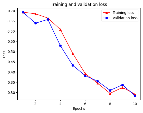
plt.plot(epochs, loss, '-r^', label='Training loss')
# "-b0" is for solid blue line with circle markers.
plt.plot(epochs, val_loss, '-bo', label='Validation loss')
plt.title('Training and validation loss')
plt.xlabel('Epochs')
plt.ylabel('Loss')
plt.legend(loc='best')
plt.show()
plt.clf()   # clear figure

plt.plot(epochs, acc, '-r^', label='Training acc')
plt.plot(epochs, val_acc, '-bo', label='Validation acc')
plt.title('Training and validation accuracy')
plt.xlabel('Epochs')
plt.ylabel('Accuracy')
plt.legend(loc='best')

plt.show()
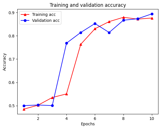
請注意,訓練損失會隨著每個週期減少,而訓練準確度會隨著每個週期增加。這是使用梯度下降最佳化時預期的結果 -- 它應該在每次迭代中最小化所需的量。
圖形正規化
我們現在準備好使用我們上面建構的基礎模型來嘗試圖形正規化。我們將使用神經結構化學習架構提供的 GraphRegularization 包裝函式類別來包裝基礎 (雙向 LSTM) 模型,以包含圖形正規化。圖形正規化模型的訓練和評估的其餘步驟與基礎模型相似。
建立圖形正規化模型
為了評估圖形正規化的增量效益,我們將建立新的基礎模型執行個體。這是因為 model 已經過幾次迭代的訓練,並且重複使用此訓練模型來建立圖形正規化模型對於 model 來說是不公平的比較。
# Build a new base LSTM model.
base_reg_model = make_bilstm_model()
# Wrap the base model with graph regularization.
graph_reg_config = nsl.configs.make_graph_reg_config(
    max_neighbors=HPARAMS.num_neighbors,
    multiplier=HPARAMS.graph_regularization_multiplier,
    distance_type=HPARAMS.distance_type,
    sum_over_axis=-1)
graph_reg_model = nsl.keras.GraphRegularization(base_reg_model,
                                                graph_reg_config)
graph_reg_model.compile(
    optimizer='adam',
    loss=tf.keras.losses.BinaryCrossentropy(from_logits=True),
    metrics=['accuracy'])
訓練模型
graph_reg_history = graph_reg_model.fit(
    train_dataset,
    validation_data=validation_dataset,
    epochs=HPARAMS.train_epochs,
    verbose=1)
Epoch 1/10
WARNING:tensorflow:From /tmpfs/src/tf_docs_env/lib/python3.9/site-packages/tensorflow/python/autograph/pyct/static_analysis/liveness.py:83: Analyzer.lamba_check (from tensorflow.python.autograph.pyct.static_analysis.liveness) is deprecated and will be removed after 2023-09-23.
Instructions for updating:
Lambda fuctions will be no more assumed to be used in the statement where they are used, or at least in the same block. https://github.com/tensorflow/tensorflow/issues/56089
21/21 [==============================] - 27s 920ms/step - loss: 0.6938 - accuracy: 0.4858 - scaled_graph_loss: 3.3994e-05 - val_loss: 0.6928 - val_accuracy: 0.5024
Epoch 2/10
21/21 [==============================] - 17s 836ms/step - loss: 0.6921 - accuracy: 0.5085 - scaled_graph_loss: 2.2528e-05 - val_loss: 0.6916 - val_accuracy: 0.4987
Epoch 3/10
21/21 [==============================] - 18s 844ms/step - loss: 0.6806 - accuracy: 0.5088 - scaled_graph_loss: 0.0018 - val_loss: 0.6383 - val_accuracy: 0.6404
Epoch 4/10
21/21 [==============================] - 17s 837ms/step - loss: 0.6143 - accuracy: 0.6588 - scaled_graph_loss: 0.0292 - val_loss: 0.5993 - val_accuracy: 0.5436
Epoch 5/10
21/21 [==============================] - 17s 841ms/step - loss: 0.5748 - accuracy: 0.7015 - scaled_graph_loss: 0.0563 - val_loss: 0.4726 - val_accuracy: 0.8239
Epoch 6/10
21/21 [==============================] - 18s 847ms/step - loss: 0.5366 - accuracy: 0.8019 - scaled_graph_loss: 0.0681 - val_loss: 0.4708 - val_accuracy: 0.7508
Epoch 7/10
21/21 [==============================] - 18s 847ms/step - loss: 0.5330 - accuracy: 0.7992 - scaled_graph_loss: 0.0722 - val_loss: 0.4462 - val_accuracy: 0.8373
Epoch 8/10
21/21 [==============================] - 18s 848ms/step - loss: 0.5207 - accuracy: 0.8096 - scaled_graph_loss: 0.0755 - val_loss: 0.4772 - val_accuracy: 0.7738
Epoch 9/10
21/21 [==============================] - 18s 851ms/step - loss: 0.5139 - accuracy: 0.8319 - scaled_graph_loss: 0.0831 - val_loss: 0.4223 - val_accuracy: 0.8412
Epoch 10/10
21/21 [==============================] - 18s 851ms/step - loss: 0.4959 - accuracy: 0.8377 - scaled_graph_loss: 0.0813 - val_loss: 0.4332 - val_accuracy: 0.8199
評估模型
graph_reg_results = graph_reg_model.evaluate(test_dataset, steps=HPARAMS.eval_steps)
print(graph_reg_results)
196/196 [==============================] - 15s 70ms/step - loss: 0.4728 - accuracy: 0.7732
[0.4728052020072937, 0.7731599807739258]
建立準確度/損失隨時間變化的圖形
graph_reg_history_dict = graph_reg_history.history
graph_reg_history_dict.keys()
dict_keys(['loss', 'accuracy', 'scaled_graph_loss', 'val_loss', 'val_accuracy'])
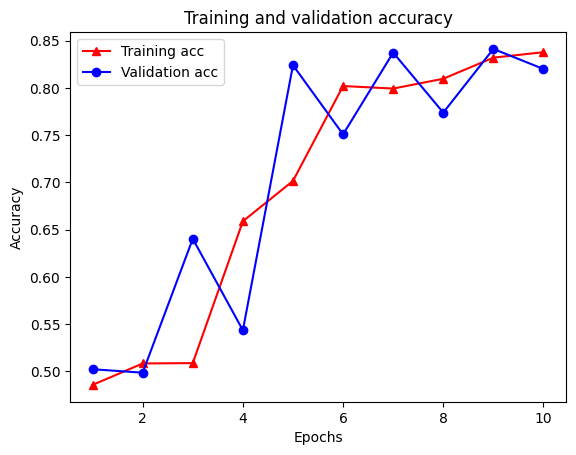
字典中總共有五個項目:訓練損失、訓練準確度、訓練圖形損失、驗證損失和驗證準確度。我們可以將它們全部繪製在一起進行比較。請注意,圖形損失僅在訓練期間計算。
acc = graph_reg_history_dict['accuracy']
val_acc = graph_reg_history_dict['val_accuracy']
loss = graph_reg_history_dict['loss']
graph_loss = graph_reg_history_dict['scaled_graph_loss']
val_loss = graph_reg_history_dict['val_loss']

epochs = range(1, len(acc) + 1)

plt.clf()   # clear figure

# "-r^" is for solid red line with triangle markers.
plt.plot(epochs, loss, '-r^', label='Training loss')
# "-gD" is for solid green line with diamond markers.
plt.plot(epochs, graph_loss, '-gD', label='Training graph loss')
# "-b0" is for solid blue line with circle markers.
plt.plot(epochs, val_loss, '-bo', label='Validation loss')
plt.title('Training and validation loss')
plt.xlabel('Epochs')
plt.ylabel('Loss')
plt.legend(loc='best')

plt.show()

plt.clf()   # clear figure

plt.plot(epochs, acc, '-r^', label='Training acc')
plt.plot(epochs, val_acc, '-bo', label='Validation acc')
plt.title('Training and validation accuracy')
plt.xlabel('Epochs')
plt.ylabel('Accuracy')
plt.legend(loc='best')

plt.show()
半監督式學習的力量
半監督式學習,更具體地說,在本教學課程的背景下,圖形正規化在訓練資料量小時可能非常強大。訓練資料的缺乏會透過利用訓練範例之間的相似度來彌補,這在傳統的監督式學習中是不可能的。
我們將監督比例定義為訓練範例與樣本總數 (包括訓練、驗證和測試樣本) 的比率。在本筆記本中,我們對基礎模型和圖形正規化模型都使用了 0.05 的監督比例 (即 5% 的標記資料) 進行訓練。我們在下面的儲存格中說明監督比例對模型準確度的影響。
# Accuracy values for both the Bi-LSTM model and the feed forward NN model have
# been precomputed for the following supervision ratios.

supervision_ratios = [0.3, 0.15, 0.05, 0.03, 0.02, 0.01, 0.005]

model_tags = ['Bi-LSTM model', 'Feed Forward NN model']
base_model_accs = [[84, 84, 83, 80, 65, 52, 50], [87, 86, 76, 74, 67, 52, 51]]
graph_reg_model_accs = [[84, 84, 83, 83, 65, 63, 50],
                        [87, 86, 80, 75, 67, 52, 50]]

plt.clf()  # clear figure

fig, axes = plt.subplots(1, 2)
fig.set_size_inches((12, 5))

for ax, model_tag, base_model_acc, graph_reg_model_acc in zip(
    axes, model_tags, base_model_accs, graph_reg_model_accs):

  # "-r^" is for solid red line with triangle markers.
  ax.plot(base_model_acc, '-r^', label='Base model')
  # "-gD" is for solid green line with diamond markers.
  ax.plot(graph_reg_model_acc, '-gD', label='Graph-regularized model')
  ax.set_title(model_tag)
  ax.set_xlabel('Supervision ratio')
  ax.set_ylabel('Accuracy(%)')
  ax.set_ylim((25, 100))
  ax.set_xticks(range(len(supervision_ratios)))
  ax.set_xticklabels(supervision_ratios)
  ax.legend(loc='best')

plt.show()
<Figure size 640x480 with 0 Axes>
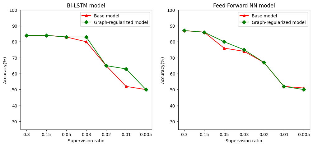
可以觀察到,隨著監督比例的降低,模型準確度也會降低。無論使用的模型架構為何,基礎模型和圖形正規化模型都是如此。但是,請注意,對於這兩種架構,圖形正規化模型的效能都優於基礎模型。特別是,對於 Bi-LSTM 模型,當監督比例為 0.01 時,圖形正規化模型的準確度比基礎模型高出 ~20%。這主要是因為圖形正規化模型的半監督式學習,其中除了訓練範例本身之外,還使用了訓練範例之間的結構相似度。
結論
即使在輸入不包含明確圖形的情況下,我們也示範了如何使用神經結構化學習 (NSL) 架構進行圖形正規化。我們考慮了 IMDB 電影評論的情感分類任務,為此我們根據評論嵌入合成了一個相似度圖形。我們鼓勵使用者透過改變超參數、監督量以及使用不同的模型架構來進一步實驗。