
|
|
|
 在 GitHub 上檢視原始碼 在 GitHub 上檢視原始碼
|
|
TensorFlow Quantum 將量子基本概念導入 TensorFlow 生態系統。現在,量子研究人員可以運用 TensorFlow 的工具。在本教學課程中,您將更深入瞭解如何將 TensorBoard 納入量子運算研究。使用 TensorFlow 的 DCGAN 教學課程,您將快速建立可運作的實驗和視覺化內容,類似於 Niu 等人所做的實驗和視覺化內容。廣義來說,您將:
- 訓練 GAN,以產生看起來像是來自量子電路的樣本。
- 視覺化訓練進度以及分佈隨時間的演變。
- 透過探索運算圖來評估實驗效能。
pip install tensorflow==2.15.0 tensorflow-quantum==0.7.3 tensorboard_plugin_profile==2.15.0
# Update package resources to account for version changes.
import importlib, pkg_resources
importlib.reload(pkg_resources)
/tmpfs/tmp/ipykernel_16243/1875984233.py:2: DeprecationWarning: pkg_resources is deprecated as an API. See https://setuptools.pypa.io/en/latest/pkg_resources.html
  import importlib, pkg_resources
<module 'pkg_resources' from '/tmpfs/src/tf_docs_env/lib/python3.9/site-packages/pkg_resources/__init__.py'>
#docs_infra: no_execute
%load_ext tensorboard
import datetime
import time
import cirq
import tensorflow as tf
import tensorflow_quantum as tfq
from tensorflow.keras import layers

# visualization tools
%matplotlib inline
import matplotlib.pyplot as plt
from cirq.contrib.svg import SVGCircuit
2024-05-18 11:28:15.992999: E external/local_xla/xla/stream_executor/cuda/cuda_dnn.cc:9261] Unable to register cuDNN factory: Attempting to register factory for plugin cuDNN when one has already been registered
2024-05-18 11:28:15.993049: E external/local_xla/xla/stream_executor/cuda/cuda_fft.cc:607] Unable to register cuFFT factory: Attempting to register factory for plugin cuFFT when one has already been registered
2024-05-18 11:28:15.994545: E external/local_xla/xla/stream_executor/cuda/cuda_blas.cc:1515] Unable to register cuBLAS factory: Attempting to register factory for plugin cuBLAS when one has already been registered
2024-05-18 11:28:17.993011: E external/local_xla/xla/stream_executor/cuda/cuda_driver.cc:274] failed call to cuInit: CUDA_ERROR_NO_DEVICE: no CUDA-capable device is detected
1. 資料產生
首先收集一些資料。您可以使用 TensorFlow Quantum 快速產生一些位元字串樣本,這些樣本將作為其餘實驗的主要資料來源。與 Niu 等人一樣,您將探索模擬從深度大幅降低的隨機電路取樣有多容易。首先,定義一些輔助程式
def generate_circuit(qubits):
    """Generate a random circuit on qubits."""
    random_circuit = cirq.experiments.random_rotations_between_grid_interaction_layers_circuit(
        qubits, depth=2)
    return random_circuit

def generate_data(circuit, n_samples):
    """Draw n_samples samples from circuit into a tf.Tensor."""
    return tf.squeeze(tfq.layers.Sample()(circuit, repetitions=n_samples).to_tensor())
現在您可以檢查電路以及一些範例資料
qubits = cirq.GridQubit.rect(1, 5)
random_circuit_m = generate_circuit(qubits) + cirq.measure_each(*qubits)
SVGCircuit(random_circuit_m)
findfont: Font family 'Arial' not found.
findfont: Font family 'Arial' not found.
findfont: Font family 'Arial' not found.
findfont: Font family 'Arial' not found.
findfont: Font family 'Arial' not found.
findfont: Font family 'Arial' not found.
findfont: Font family 'Arial' not found.
findfont: Font family 'Arial' not found.
findfont: Font family 'Arial' not found.
findfont: Font family 'Arial' not found.
findfont: Font family 'Arial' not found.
findfont: Font family 'Arial' not found.
findfont: Font family 'Arial' not found.
findfont: Font family 'Arial' not found.
findfont: Font family 'Arial' not found.
findfont: Font family 'Arial' not found.
findfont: Font family 'Arial' not found.
findfont: Font family 'Arial' not found.
findfont: Font family 'Arial' not found.
findfont: Font family 'Arial' not found.
findfont: Font family 'Arial' not found.
findfont: Font family 'Arial' not found.
findfont: Font family 'Arial' not found.
findfont: Font family 'Arial' not found.
findfont: Font family 'Arial' not found.

samples = cirq.sample(random_circuit_m, repetitions=10)
print('10 Random bitstrings from this circuit:')
print(samples)
10 Random bitstrings from this circuit:
q(0, 0)=1011111111
q(0, 1)=1111111111
q(0, 2)=1011111111
q(0, 3)=0100010111
q(0, 4)=1111111101
您可以使用 TensorFlow Quantum 執行相同的操作:
generate_data(random_circuit_m, 10)
<tf.Tensor: shape=(10, 5), dtype=int8, numpy=
array([[0, 1, 1, 1, 1],
       [1, 1, 1, 0, 1],
       [1, 1, 1, 0, 1],
       [1, 1, 1, 0, 1],
       [1, 1, 1, 1, 1],
       [1, 1, 1, 1, 1],
       [1, 1, 1, 1, 1],
       [1, 1, 1, 1, 1],
       [1, 1, 1, 1, 1],
       [1, 1, 1, 1, 1]], dtype=int8)>
現在您可以快速產生訓練資料:
N_SAMPLES = 60000
N_QUBITS = 10
QUBITS = cirq.GridQubit.rect(1, N_QUBITS)
REFERENCE_CIRCUIT = generate_circuit(QUBITS)
all_data = generate_data(REFERENCE_CIRCUIT, N_SAMPLES)
all_data
<tf.Tensor: shape=(60000, 10), dtype=int8, numpy=
array([[0, 1, 0, ..., 1, 1, 1],
       [0, 1, 0, ..., 1, 1, 0],
       [0, 1, 0, ..., 1, 1, 0],
       ...,
       [1, 1, 1, ..., 1, 1, 1],
       [1, 1, 1, ..., 1, 1, 1],
       [1, 1, 1, ..., 1, 1, 1]], dtype=int8)>
定義一些輔助函式來視覺化訓練的進行會很有用。兩個有趣的量值是:
- 樣本的整數值,以便您可以建立分佈的直方圖。
- 樣本集的 線性 XEB 保真度估計值,以指示樣本「真實量子隨機」的程度。
@tf.function
def bits_to_ints(bits):
    """Convert tensor of bitstrings to tensor of ints."""
    sigs = tf.constant([1 << i for i in range(N_QUBITS)], dtype=tf.int32)
    rounded_bits = tf.clip_by_value(tf.math.round(
        tf.cast(bits, dtype=tf.dtypes.float32)), clip_value_min=0, clip_value_max=1)
    return tf.einsum('jk,k->j', tf.cast(rounded_bits, dtype=tf.dtypes.int32), sigs)

@tf.function
def xeb_fid(bits):
    """Compute linear XEB fidelity of bitstrings."""
    final_probs = tf.squeeze(
        tf.abs(tfq.layers.State()(REFERENCE_CIRCUIT).to_tensor()) ** 2)
    nums = bits_to_ints(bits)
    return (2 ** N_QUBITS) * tf.reduce_mean(tf.gather(final_probs, nums)) - 1.0
您可以在此處視覺化您的分佈,並使用 XEB 進行健全性檢查
plt.hist(bits_to_ints(all_data).numpy(), 50)
plt.show()
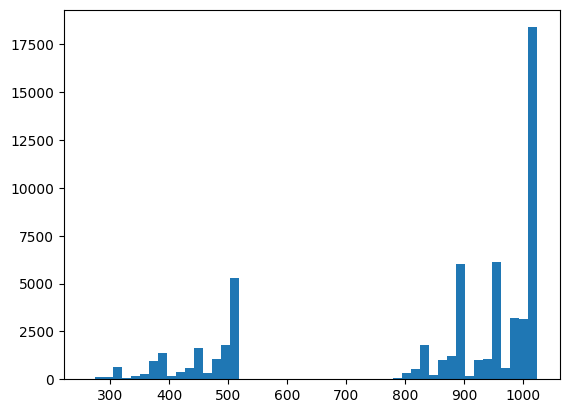
xeb_fid(all_data)
WARNING:tensorflow:You are casting an input of type complex64 to an incompatible dtype float32.  This will discard the imaginary part and may not be what you intended.
<tf.Tensor: shape=(), dtype=float32, numpy=46.323647>
2. 建立模型
您可以在此處使用 DCGAN 教學課程中的相關元件來處理量子案例。新的 GAN 不會產生 MNIST 數字,而是會用於產生長度為 N_QUBITS 的位元字串樣本
LATENT_DIM = 100
def make_generator_model():
    """Construct generator model."""
    model = tf.keras.Sequential()
    model.add(layers.Dense(256, use_bias=False, input_shape=(LATENT_DIM,)))
    model.add(layers.Dense(128, activation='relu'))
    model.add(layers.Dropout(0.3))
    model.add(layers.Dense(64, activation='relu'))
    model.add(layers.Dense(N_QUBITS, activation='relu'))

    return model

def make_discriminator_model():
    """Constrcut discriminator model."""
    model = tf.keras.Sequential()
    model.add(layers.Dense(256, use_bias=False, input_shape=(N_QUBITS,)))
    model.add(layers.Dense(128, activation='relu'))
    model.add(layers.Dropout(0.3))
    model.add(layers.Dense(32, activation='relu'))
    model.add(layers.Dense(1))

    return model
接下來,例項化您的產生器和鑑別器模型、定義損失,並建立用於主要訓練迴圈的 train_step 函式
discriminator = make_discriminator_model()
generator = make_generator_model()
cross_entropy = tf.keras.losses.BinaryCrossentropy(from_logits=True)
def discriminator_loss(real_output, fake_output):
    """Compute discriminator loss."""
    real_loss = cross_entropy(tf.ones_like(real_output), real_output)
    fake_loss = cross_entropy(tf.zeros_like(fake_output), fake_output)
    total_loss = real_loss + fake_loss
    return total_loss

def generator_loss(fake_output):
    """Compute generator loss."""
    return cross_entropy(tf.ones_like(fake_output), fake_output)

generator_optimizer = tf.keras.optimizers.Adam(1e-4)
discriminator_optimizer = tf.keras.optimizers.Adam(1e-4)
BATCH_SIZE=256

@tf.function
def train_step(images):
    """Run train step on provided image batch."""
    noise = tf.random.normal([BATCH_SIZE, LATENT_DIM])
    with tf.GradientTape() as gen_tape, tf.GradientTape() as disc_tape:
        generated_images = generator(noise, training=True)

        real_output = discriminator(images, training=True)
        fake_output = discriminator(generated_images, training=True)

        gen_loss = generator_loss(fake_output)
        disc_loss = discriminator_loss(real_output, fake_output)

    gradients_of_generator = gen_tape.gradient(
        gen_loss, generator.trainable_variables)
    gradients_of_discriminator = disc_tape.gradient(
        disc_loss, discriminator.trainable_variables)

    generator_optimizer.apply_gradients(
        zip(gradients_of_generator, generator.trainable_variables))
    discriminator_optimizer.apply_gradients(
        zip(gradients_of_discriminator, discriminator.trainable_variables))

    return gen_loss, disc_loss
現在您已具備模型所需的所有建構區塊,您可以設定包含 TensorBoard 視覺化的訓練函式。首先設定 TensorBoard 檔案寫入器
logdir = "tb_logs/" + datetime.datetime.now().strftime("%Y%m%d-%H%M%S")
file_writer = tf.summary.create_file_writer(logdir + "/metrics")
file_writer.set_as_default()
使用 tf.summary 模組,您現在可以在主要 train 函式內將 scalar、histogram (以及其他) 記錄納入 TensorBoard
def train(dataset, epochs, start_epoch=1):
    """Launch full training run for the given number of epochs."""
    # Log original training distribution.
    tf.summary.histogram('Training Distribution', data=bits_to_ints(dataset), step=0)

    batched_data = tf.data.Dataset.from_tensor_slices(dataset).shuffle(N_SAMPLES).batch(512)
    t = time.time()
    for epoch in range(start_epoch, start_epoch + epochs):
        for i, image_batch in enumerate(batched_data):
            # Log batch-wise loss.
            gl, dl = train_step(image_batch)
            tf.summary.scalar(
                'Generator loss', data=gl, step=epoch * len(batched_data) + i)
            tf.summary.scalar(
                'Discriminator loss', data=dl, step=epoch * len(batched_data) + i)

        # Log full dataset XEB Fidelity and generated distribution.
        generated_samples = generator(tf.random.normal([N_SAMPLES, 100]))
        tf.summary.scalar(
        'Generator XEB Fidelity Estimate', data=xeb_fid(generated_samples), step=epoch)
        tf.summary.histogram(
        'Generator distribution', data=bits_to_ints(generated_samples), step=epoch)
        # Log new samples drawn from this particular random circuit.
        random_new_distribution = generate_data(REFERENCE_CIRCUIT, N_SAMPLES)
        tf.summary.histogram(
        'New round of True samples', data=bits_to_ints(random_new_distribution), step=epoch)

        if epoch % 10 == 0:
            print('Epoch {}, took {}(s)'.format(epoch, time.time() - t))
            t = time.time()
3. 視覺化訓練和效能
現在可以使用以下命令啟動 TensorBoard 資訊主頁:
#docs_infra: no_execute
%tensorboard --logdir tb_logs/
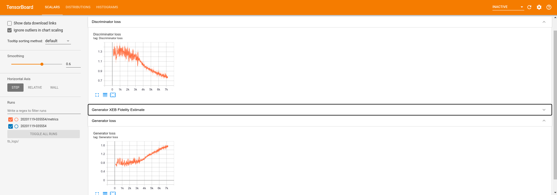
當呼叫 train 時,TensoBoard 資訊主頁將使用訓練迴圈中提供的所有摘要統計資料自動更新。
train(all_data, epochs=50)
Epoch 10, took 8.953658819198608(s)
Epoch 20, took 6.647485971450806(s)
Epoch 30, took 6.6542747020721436(s)
Epoch 40, took 6.638120889663696(s)
Epoch 50, took 6.668101072311401(s)
在訓練執行期間 (以及完成後),您可以檢查純量量值
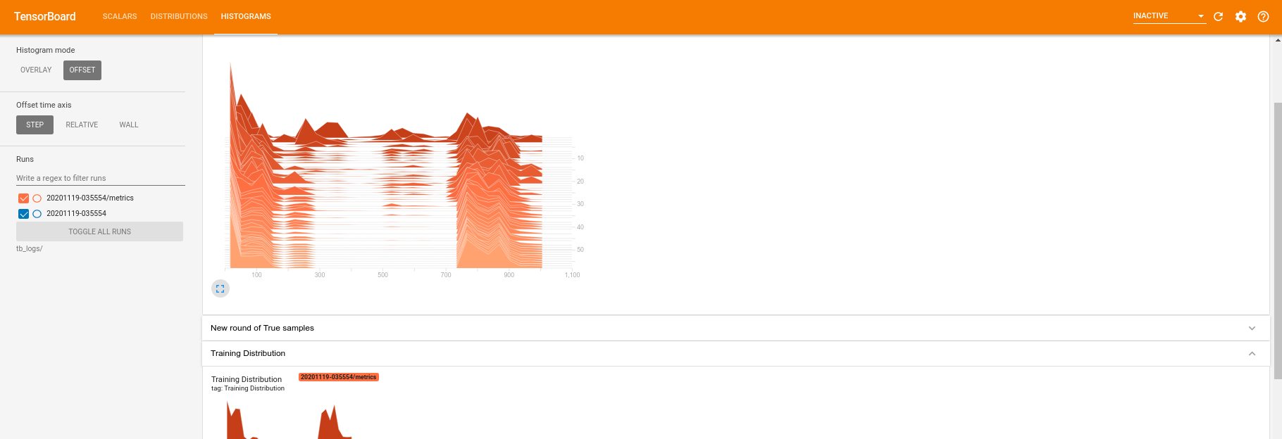
切換到直方圖分頁,您也可以查看產生器網路在重新建立量子分佈樣本方面的表現
除了允許即時監控與實驗相關的摘要統計資料外,TensorBoard 也可以協助您分析實驗效能,以找出效能瓶頸。若要使用效能監控重新執行模型,您可以執行:
tf.profiler.experimental.start(logdir)
train(all_data, epochs=10, start_epoch=50)
tf.profiler.experimental.stop()
Epoch 50, took 0.7739055156707764(s)
TensorBoard 將分析 tf.profiler.experimental.start 和 tf.profiler.experimental.stop 之間的所有程式碼。然後可以在 TensorBoard 的 profile 頁面中檢視此分析資料
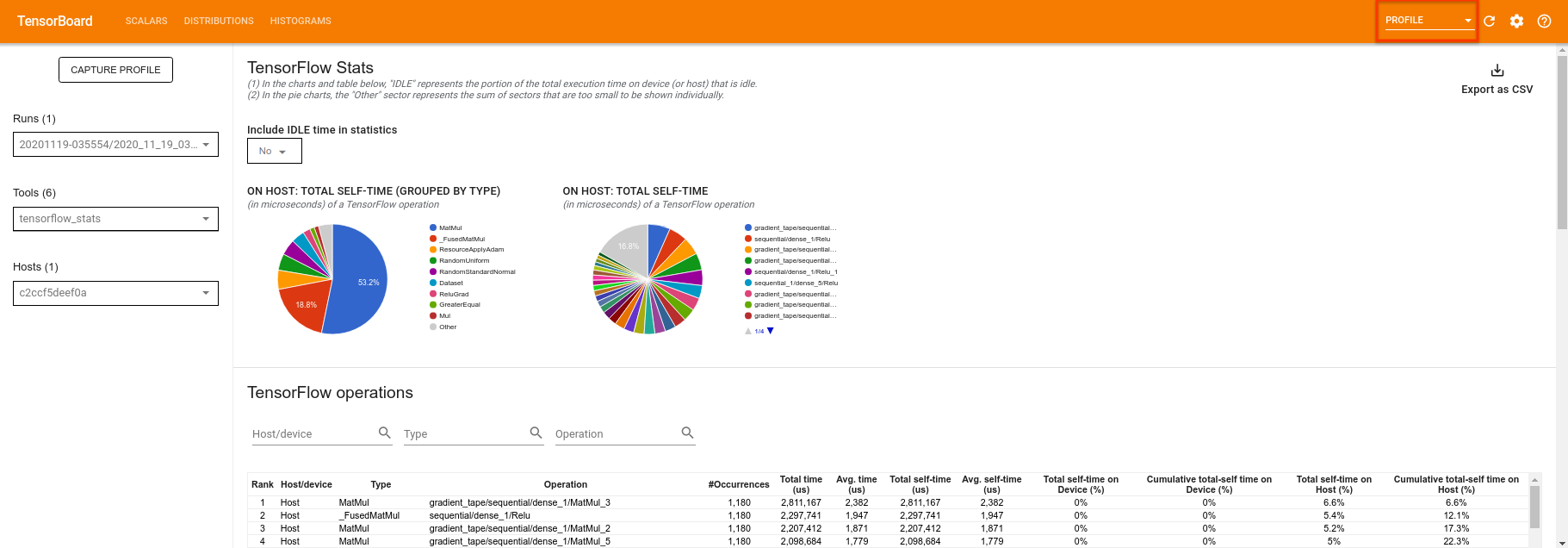
嘗試增加深度或試驗不同類型的量子電路。查看 TensorBoard 的所有其他強大功能,例如您可以納入 TensorFlow Quantum 實驗的 超參數調整。