機率圖模型上的變分推論與聯合分佈

我們使用郡縣層級的隨機效應來捕捉地理變異。參數 uranium_weight 和 county_floor_weight 以機率方式建模，而 floor_weight 和常數 bias 則是確定性的。這些建模選擇在很大程度上是任意的，並且是為了在具有合理複雜度的機率模型上示範 VI 而做出的。如需更深入討論在 TFP 中使用固定效應和隨機效應進行多層次建模（使用氡氣資料集），請參閱 Multilevel Modeling Primer 和 Fitting Generalized Linear Mixed-effects Models Using Variational Inference。

# Create variables for fixed effects.
floor_weight = tf.Variable(0.)
bias = tf.Variable(0.)

# Variables for scale parameters.
log_radon_scale = tfp.util.TransformedVariable(1., tfb.Exp())
county_effect_scale = tfp.util.TransformedVariable(1., tfb.Exp())

# Define the probabilistic graphical model as a JointDistribution.
@tfd.JointDistributionCoroutineAutoBatched
def model():
  uranium_weight = yield tfd.Normal(0., scale=1., name='uranium_weight')
  county_floor_weight = yield tfd.Normal(
      0., scale=1., name='county_floor_weight')
  county_effect = yield tfd.Sample(
      tfd.Normal(0., scale=county_effect_scale),
      sample_shape=[num_counties], name='county_effect')
  yield tfd.Normal(
      loc=(log_uranium * uranium_weight + floor_of_house* floor_weight
           + floor_by_county * county_floor_weight
           + tf.gather(county_effect, county, axis=-1)
           + bias),
      scale=log_radon_scale[..., tf.newaxis],
      name='log_radon') 

# Pin the observed `log_radon` values to model the un-normalized posterior.
target_model = model.experimental_pin(log_radon=log_radon)

表達力強的替代後驗分佈

接下來，我們使用 VI 和兩種不同類型的替代後驗分佈來估計隨機效應的後驗分佈：

• 受約束的多變數常態分佈，其共變異數結構由區塊式矩陣轉換誘導。
• 由逆自迴歸流轉換的多變數標準常態分佈，然後將其分割並重新建構以符合後驗分佈的支援。

多變數常態替代後驗分佈

為了建構此替代後驗分佈，使用可訓練的線性運算子來誘導後驗分佈組件之間的相關性。

# Determine the `event_shape` of the posterior, and calculate the size of each
# `event_shape` component. These determine the sizes of the components of the
# underlying standard Normal distribution, and the dimensions of the blocks in
# the blockwise matrix transformation.
event_shape = target_model.event_shape_tensor()
flat_event_shape = tf.nest.flatten(event_shape)
flat_event_size = tf.nest.map_structure(tf.reduce_prod, flat_event_shape)

# The `event_space_bijector` maps unconstrained values (in R^n) to the support
# of the prior -- we'll need this at the end to constrain Multivariate Normal
# samples to the prior's support.
event_space_bijector = target_model.experimental_default_event_space_bijector()

建構一個 JointDistribution，其中包含向量值標準常態組件，其大小由對應的先驗組件決定。組件應為向量值，以便可以由線性運算子轉換。

base_standard_dist = tfd.JointDistributionSequential(
      [tfd.Sample(tfd.Normal(0., 1.), s) for s in flat_event_size])

建構一個可訓練的區塊式下三角線性運算子。我們將其應用於標準常態分佈，以實作（可訓練的）區塊式矩陣轉換並誘導後驗分佈的相關結構。

在區塊式線性運算子中，可訓練的完整矩陣區塊表示後驗分佈的兩個組件之間的完全共變異數，而零區塊（或 None）則表示獨立性。對角線上的區塊可以是下三角矩陣或對角矩陣，因此整個區塊結構代表下三角矩陣。

將此雙射器應用於基礎分佈會產生一個平均值為 0 且（Cholesky 分解）共變異數等於下三角區塊矩陣的多變數常態分佈。

operators = (
    (tf.linalg.LinearOperatorDiag,),  # Variance of uranium weight (scalar).
    (tf.linalg.LinearOperatorFullMatrix,  # Covariance between uranium and floor-by-county weights.
     tf.linalg.LinearOperatorDiag),  # Variance of floor-by-county weight (scalar).
    (None,  # Independence between uranium weight and county effects.
     None,  #  Independence between floor-by-county and county effects.
     tf.linalg.LinearOperatorDiag)  # Independence among the 85 county effects.
    )

block_tril_linop = (
    tfp.experimental.vi.util.build_trainable_linear_operator_block(
        operators, flat_event_size))
scale_bijector = tfb.ScaleMatvecLinearOperatorBlock(block_tril_linop)

將線性運算子應用於標準常態分佈後，應用多部分 Shift 雙射器以允許平均值取非零值。

loc_bijector = tfb.JointMap(
    tf.nest.map_structure(
        lambda s: tfb.Shift(
            tf.Variable(tf.random.uniform(
                (s,), minval=-2., maxval=2., dtype=tf.float32))),
        flat_event_size))

通過使用尺度和位置雙射器轉換標準常態分佈而獲得的最終多變數常態分佈，必須重新調整形狀和重新建構以符合先驗分佈，並最終約束到先驗分佈的支援。

# Reshape each component to match the prior, using a nested structure of
# `Reshape` bijectors wrapped in `JointMap` to form a multipart bijector.
reshape_bijector = tfb.JointMap(
    tf.nest.map_structure(tfb.Reshape, flat_event_shape))

# Restructure the flat list of components to match the prior's structure
unflatten_bijector = tfb.Restructure(
        tf.nest.pack_sequence_as(
            event_shape, range(len(flat_event_shape))))

現在，將所有內容放在一起——將可訓練的雙射器鏈結在一起，並將它們應用於基礎標準常態分佈，以建構替代後驗分佈。

surrogate_posterior = tfd.TransformedDistribution(
    base_standard_dist,
    bijector = tfb.Chain(  # Note that the chained bijectors are applied in reverse order
        [
         event_space_bijector,  # constrain the surrogate to the support of the prior
         unflatten_bijector,  # pack the reshaped components into the `event_shape` structure of the posterior
         reshape_bijector,  # reshape the vector-valued components to match the shapes of the posterior components
         loc_bijector,  # allow for nonzero mean
         scale_bijector  # apply the block matrix transformation to the standard Normal distribution
         ]))

訓練多變數常態替代後驗分佈。

optimizer = tf_keras.optimizers.Adam(learning_rate=1e-2)
mvn_loss = tfp.vi.fit_surrogate_posterior(
    target_model.unnormalized_log_prob,
    surrogate_posterior,
    optimizer=optimizer,
    num_steps=10**4,
    sample_size=16,
    jit_compile=True)

mvn_samples = surrogate_posterior.sample(1000)
mvn_final_elbo = tf.reduce_mean(
    target_model.unnormalized_log_prob(*mvn_samples)
    - surrogate_posterior.log_prob(mvn_samples))

print('Multivariate Normal surrogate posterior ELBO: {}'.format(mvn_final_elbo))

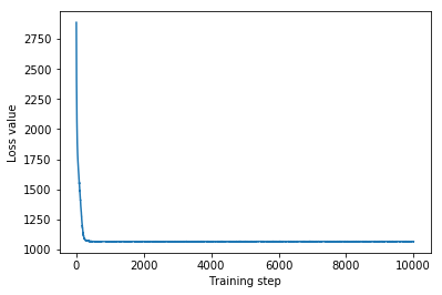
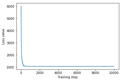
plt.plot(mvn_loss)
plt.xlabel('Training step')
_ = plt.ylabel('Loss value')

Multivariate Normal surrogate posterior ELBO: -1065.705322265625

由於訓練後的替代後驗分佈是 TFP 分佈，我們可以從中取樣並處理它們，以產生參數的後驗可信區間。

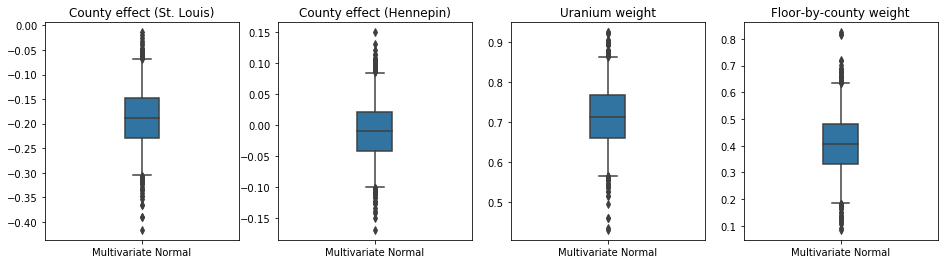
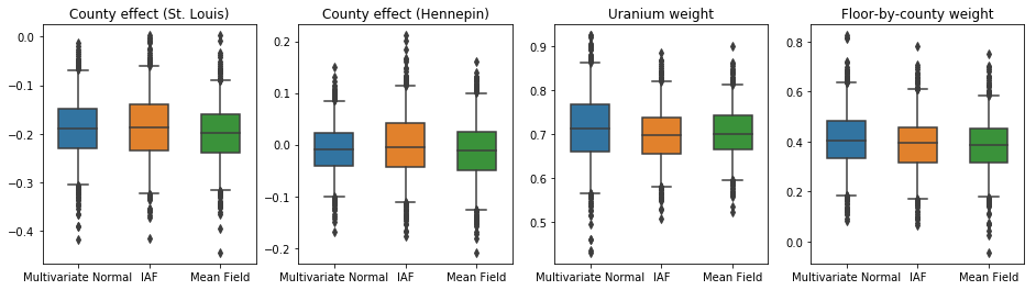
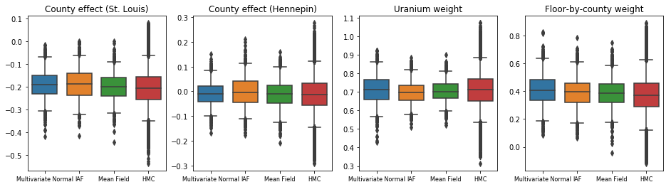
下方的盒鬚圖顯示了兩個最大郡縣的郡縣效應以及土壤鈾測量值和按郡縣劃分的平均樓層的迴歸權重的 50% 和 95% 可信區間。郡縣效應的後驗可信區間表示，在考慮其他變數後，聖路易郡的位置與較低的氡氣濃度相關，而亨內平郡的位置效應接近中性。

迴歸權重的後驗可信區間顯示，較高的土壤鈾濃度與較高的氡氣濃度相關，並且在較高樓層進行測量的郡縣（可能是因為房屋沒有地下室）往往具有較高的氡氣濃度，這可能與土壤特性及其對建築結構類型的影響有關。

樓層的（確定性）係數為負，表示較低樓層的氡氣濃度較高，正如預期的那樣。

st_louis_co = 69  # Index of St. Louis, the county with the most observations.
hennepin_co = 25  # Index of Hennepin, with the second-most observations.

def pack_samples(samples):
  return {'County effect (St. Louis)': samples.county_effect[..., st_louis_co],
          'County effect (Hennepin)': samples.county_effect[..., hennepin_co],
          'Uranium weight': samples.uranium_weight,
          'Floor-by-county weight': samples.county_floor_weight}

def plot_boxplot(posterior_samples):
  fig, axes = plt.subplots(1, 4, figsize=(16, 4))

  # Invert the results dict for easier plotting.
  k = list(posterior_samples.values())[0].keys()
  plot_results = {
      v: {p: posterior_samples[p][v] for p in posterior_samples} for v in k}
  for i, (var, var_results) in enumerate(plot_results.items()):
    sns.boxplot(data=list(var_results.values()), ax=axes[i],
                width=0.18*len(var_results), whis=(2.5, 97.5))
    # axes[i].boxplot(list(var_results.values()), whis=(2.5, 97.5))
    axes[i].title.set_text(var)
    fs = 10 if len(var_results) < 4 else 8
    axes[i].set_xticklabels(list(var_results.keys()), fontsize=fs)

results = {'Multivariate Normal': pack_samples(mvn_samples)}

print('Bias is: {:.2f}'.format(bias.numpy()))
print('Floor fixed effect is: {:.2f}'.format(floor_weight.numpy()))
plot_boxplot(results)

Bias is: 1.40
Floor fixed effect is: -0.72

逆自迴歸流替代後驗分佈

逆自迴歸流 (IAF) 是正規化流，它使用神經網路來捕捉分佈組件之間複雜的非線性依賴性。接下來，我們建構一個 IAF 替代後驗分佈，以查看此更高容量、更靈活的模型是否優於受約束的多變數常態分佈。

# Build a standard Normal with a vector `event_shape`, with length equal to the
# total number of degrees of freedom in the posterior.
base_distribution = tfd.Sample(
    tfd.Normal(0., 1.), sample_shape=[tf.reduce_sum(flat_event_size)])

# Apply an IAF to the base distribution.
num_iafs = 2
iaf_bijectors = [
    tfb.Invert(tfb.MaskedAutoregressiveFlow(
        shift_and_log_scale_fn=tfb.AutoregressiveNetwork(
            params=2, hidden_units=[256, 256], activation='relu')))
    for _ in range(num_iafs)
]

# Split the base distribution's `event_shape` into components that are equal
# in size to the prior's components.
split = tfb.Split(flat_event_size)

# Chain these bijectors and apply them to the standard Normal base distribution
# to build the surrogate posterior. `event_space_bijector`,
# `unflatten_bijector`, and `reshape_bijector` are the same as in the
# multivariate Normal surrogate posterior.
iaf_surrogate_posterior = tfd.TransformedDistribution(
    base_distribution,
    bijector=tfb.Chain([
         event_space_bijector,  # constrain the surrogate to the support of the prior
         unflatten_bijector,  # pack the reshaped components into the `event_shape` structure of the prior
         reshape_bijector,  # reshape the vector-valued components to match the shapes of the prior components
         split] +  # Split the samples into components of the same size as the prior components
         iaf_bijectors  # Apply a flow model to the Tensor-valued standard Normal distribution
         ))

訓練 IAF 替代後驗分佈。

optimizer=tf_keras.optimizers.Adam(learning_rate=1e-2)
iaf_loss = tfp.vi.fit_surrogate_posterior(
  target_model.unnormalized_log_prob,
  iaf_surrogate_posterior,
  optimizer=optimizer,
  num_steps=10**4,
  sample_size=4,
  jit_compile=True)

iaf_samples = iaf_surrogate_posterior.sample(1000)
iaf_final_elbo = tf.reduce_mean(
    target_model.unnormalized_log_prob(*iaf_samples)
    - iaf_surrogate_posterior.log_prob(iaf_samples))
print('IAF surrogate posterior ELBO: {}'.format(iaf_final_elbo))

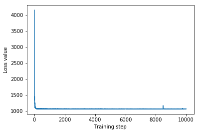
plt.plot(iaf_loss)
plt.xlabel('Training step')
_ = plt.ylabel('Loss value')

IAF surrogate posterior ELBO: -1065.3663330078125

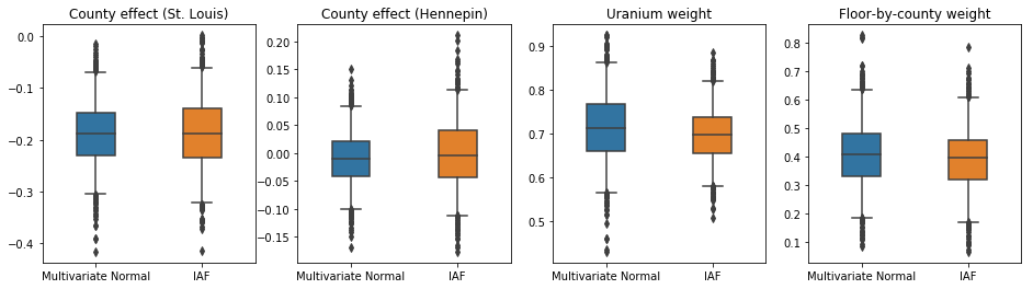
IAF 替代後驗分佈的可信區間似乎與受約束的多變數常態分佈的可信區間相似。

results['IAF'] = pack_samples(iaf_samples)
plot_boxplot(results)

基準線：平均場替代後驗分佈

VI 替代後驗分佈通常被假設為平均場（獨立）常態分佈，具有可訓練的平均值和變異數，這些分佈通過雙射轉換約束到先驗分佈的支援。除了兩個更具表達力的替代後驗分佈之外，我們還定義了一個平均場替代後驗分佈，使用與多變數常態替代後驗分佈相同的通用公式。

# A block-diagonal linear operator, in which each block is a diagonal operator,
# transforms the standard Normal base distribution to produce a mean-field
# surrogate posterior.
operators = (tf.linalg.LinearOperatorDiag,
             tf.linalg.LinearOperatorDiag,
             tf.linalg.LinearOperatorDiag)
block_diag_linop = (
    tfp.experimental.vi.util.build_trainable_linear_operator_block(
        operators, flat_event_size))
mean_field_scale = tfb.ScaleMatvecLinearOperatorBlock(block_diag_linop)

mean_field_loc = tfb.JointMap(
    tf.nest.map_structure(
        lambda s: tfb.Shift(
            tf.Variable(tf.random.uniform(
                (s,), minval=-2., maxval=2., dtype=tf.float32))),
        flat_event_size))

mean_field_surrogate_posterior = tfd.TransformedDistribution(
    base_standard_dist,
    bijector = tfb.Chain(  # Note that the chained bijectors are applied in reverse order
        [
         event_space_bijector,  # constrain the surrogate to the support of the prior
         unflatten_bijector,  # pack the reshaped components into the `event_shape` structure of the posterior
         reshape_bijector, # reshape the vector-valued components to match the shapes of the posterior components
         mean_field_loc,   # allow for nonzero mean
         mean_field_scale  # apply the block matrix transformation to the standard Normal distribution
         ]))

optimizer=tf_keras.optimizers.Adam(learning_rate=1e-2)
mean_field_loss = tfp.vi.fit_surrogate_posterior(
    target_model.unnormalized_log_prob,
    mean_field_surrogate_posterior,
    optimizer=optimizer,
    num_steps=10**4,
    sample_size=16,
    jit_compile=True)

mean_field_samples = mean_field_surrogate_posterior.sample(1000)
mean_field_final_elbo = tf.reduce_mean(
    target_model.unnormalized_log_prob(*mean_field_samples)
    - mean_field_surrogate_posterior.log_prob(mean_field_samples))
print('Mean-field surrogate posterior ELBO: {}'.format(mean_field_final_elbo))

plt.plot(mean_field_loss)
plt.xlabel('Training step')
_ = plt.ylabel('Loss value')

Mean-field surrogate posterior ELBO: -1065.7652587890625

在這種情況下，平均場替代後驗分佈給出的結果與更具表達力的替代後驗分佈相似，這表示此較簡單的模型可能足以用於推論任務。

results['Mean Field'] = pack_samples(mean_field_samples)
plot_boxplot(results)

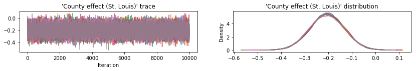
地面實況：哈密頓蒙地卡羅 (HMC)

我們使用 HMC 從真實後驗分佈生成「地面實況」樣本，以便與替代後驗分佈的結果進行比較。

num_chains = 8
num_leapfrog_steps = 3
step_size = 0.4
num_steps=20000

flat_event_shape = tf.nest.flatten(target_model.event_shape)
enum_components = list(range(len(flat_event_shape)))
bijector = tfb.Restructure(
    enum_components,
    tf.nest.pack_sequence_as(target_model.event_shape, enum_components))(
        target_model.experimental_default_event_space_bijector())

current_state = bijector(
    tf.nest.map_structure(
        lambda e: tf.zeros([num_chains] + list(e), dtype=tf.float32),
    target_model.event_shape))

hmc = tfp.mcmc.HamiltonianMonteCarlo(
    target_log_prob_fn=target_model.unnormalized_log_prob,
    num_leapfrog_steps=num_leapfrog_steps,
    step_size=[tf.fill(s.shape, step_size) for s in current_state])

hmc = tfp.mcmc.TransformedTransitionKernel(
    hmc, bijector)
hmc = tfp.mcmc.DualAveragingStepSizeAdaptation(
    hmc,
    num_adaptation_steps=int(num_steps // 2 * 0.8),
    target_accept_prob=0.9)

chain, is_accepted = tf.function(
    lambda current_state: tfp.mcmc.sample_chain(
        current_state=current_state,
        kernel=hmc,
        num_results=num_steps // 2,
        num_burnin_steps=num_steps // 2,
        trace_fn=lambda _, pkr:
        (pkr.inner_results.inner_results.is_accepted),
        ),
    autograph=False,
    jit_compile=True)(current_state)

accept_rate = tf.reduce_mean(tf.cast(is_accepted, tf.float32))
ess = tf.nest.map_structure(
    lambda c: tfp.mcmc.effective_sample_size(
        c,
        cross_chain_dims=1,
        filter_beyond_positive_pairs=True),
    chain)

r_hat = tf.nest.map_structure(tfp.mcmc.potential_scale_reduction, chain)
hmc_samples = pack_samples(
    tf.nest.pack_sequence_as(target_model.event_shape, chain))
print('Acceptance rate is {}'.format(accept_rate))

Acceptance rate is 0.9008625149726868

繪製樣本追蹤圖以對 HMC 結果進行健全性檢查。

def plot_traces(var_name, samples):
  fig, axes = plt.subplots(1, 2, figsize=(14, 1.5), sharex='col', sharey='col')
  for chain in range(num_chains):
    s = samples.numpy()[:, chain]
    axes[0].plot(s, alpha=0.7)
    sns.kdeplot(s, ax=axes[1], shade=False)
    axes[0].title.set_text("'{}' trace".format(var_name))
    axes[1].title.set_text("'{}' distribution".format(var_name))
    axes[0].set_xlabel('Iteration')

warnings.filterwarnings('ignore')
for var, var_samples in hmc_samples.items():
  plot_traces(var, var_samples)

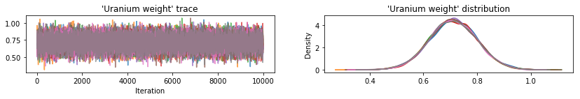
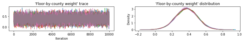
所有三個替代後驗分佈產生的可信區間在視覺上與 HMC 樣本相似，但有時由於 ELBO 損失的影響而過於分散，這在 VI 中很常見。

results['HMC'] = hmc_samples
plot_boxplot(results)

其他結果

繪圖函數

plt.rcParams.update({'axes.titlesize': 'medium', 'xtick.labelsize': 'medium'})
def plot_loss_and_elbo():
  fig, axes = plt.subplots(1, 2, figsize=(12, 4))

  axes[0].scatter([0, 1, 2],
                  [mvn_final_elbo.numpy(),
                  iaf_final_elbo.numpy(),
                  mean_field_final_elbo.numpy()])
  axes[0].set_xticks(ticks=[0, 1, 2])
  axes[0].set_xticklabels(labels=[
    'Multivariate Normal', 'IAF', 'Mean Field'])
  axes[0].title.set_text('Evidence Lower Bound (ELBO)')

  axes[1].plot(mvn_loss, label='Multivariate Normal')
  axes[1].plot(iaf_loss, label='IAF')
  axes[1].plot(mean_field_loss, label='Mean Field')
  axes[1].set_ylim([1000, 4000])
  axes[1].set_xlabel('Training step')
  axes[1].set_ylabel('Loss (negative ELBO)')
  axes[1].title.set_text('Loss')
  plt.legend()
  plt.show()

plt.rcParams.update({'axes.titlesize': 'medium', 'xtick.labelsize': 'small'})
def plot_kdes(num_chains=8):
  fig, axes = plt.subplots(2, 2, figsize=(12, 8))
  k = list(results.values())[0].keys()
  plot_results = {
      v: {p: results[p][v] for p in results} for v in k}
  for i, (var, var_results) in enumerate(plot_results.items()):
    ax = axes[i % 2, i // 2]
    for posterior, posterior_results in var_results.items():
      if posterior == 'HMC':
        label = posterior
        for chain in range(num_chains):
          sns.kdeplot(
              posterior_results[:, chain],
              ax=ax, shade=False, color='k', linestyle=':', label=label)
          label=None
      else:
        sns.kdeplot(
            posterior_results, ax=ax, shade=False, label=posterior)
        ax.title.set_text('{}'.format(var))
    ax.legend()

證據下限 (ELBO)

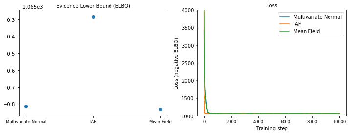
IAF 是迄今為止最大且最靈活的替代後驗分佈，它收斂到最高的證據下限 (ELBO)。

plot_loss_and_elbo()

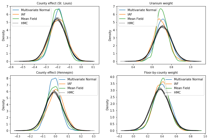
後驗樣本

來自每個替代後驗分佈的樣本，與 HMC 地面實況樣本進行比較（盒鬚圖中顯示的樣本的不同視覺化呈現）。

plot_kdes()

結論

在此 Colab 中，我們使用聯合分佈和多部分雙射器建構了 VI 替代後驗分佈，並擬合它們以估計氡氣資料集上迴歸模型中權重的可信區間。對於這個簡單的模型，更具表達力的替代後驗分佈的效能與平均場替代後驗分佈相似。然而，我們示範的工具可用於建構適用於更複雜模型的各種靈活替代後驗分佈。