
|
|
|
 在 GitHub 上檢視原始碼 在 GitHub 上檢視原始碼
|
|
TensorFlow Probability (TFP) 是一個用於機率推理和統計分析的程式庫,現在也適用於 JAX!對於不熟悉的使用者,JAX 是一個以可組合函式轉換為基礎的加速數值運算程式庫。
JAX 上的 TFP 支援常規 TFP 的許多最實用功能,同時保留許多 TFP 使用者現在已習慣的抽象概念和 API。
設定
JAX 上的 TFP 不依賴 TensorFlow;讓我們從這個 Colab 完全解除安裝 TensorFlow。
pip uninstall tensorflow -y -q
我們可以透過 TFP 的最新每夜建置版本在 JAX 上安裝 TFP。
pip install -Uq tfp-nightly[jax] > /dev/null
讓我們匯入一些實用的 Python 程式庫。
import matplotlib.pyplot as plt
import numpy as np
import seaborn as sns
from sklearn import datasets
sns.set(style='white')
/usr/local/lib/python3.6/dist-packages/statsmodels/tools/_testing.py:19: FutureWarning: pandas.util.testing is deprecated. Use the functions in the public API at pandas.testing instead.
  import pandas.util.testing as tm
我們也匯入一些基本的 JAX 功能。
import jax.numpy as jnp
from jax import grad
from jax import jit
from jax import random
from jax import value_and_grad
from jax import vmap
在 JAX 上匯入 TFP
若要在 JAX 上使用 TFP,只需匯入 jax「基底」,然後像平常一樣使用 tfp
from tensorflow_probability.substrates import jax as tfp
tfd = tfp.distributions
tfb = tfp.bijectors
tfpk = tfp.math.psd_kernels
示範:貝氏邏輯迴歸
為了示範我們可以使用 JAX 後端做什麼,我們將實作應用於經典鳶尾花資料集的貝氏邏輯迴歸。
首先,讓我們匯入鳶尾花資料集並擷取一些中繼資料。
iris = datasets.load_iris()
features, labels = iris['data'], iris['target']

num_features = features.shape[-1]
num_classes = len(iris.target_names)
我們可以使用 tfd.JointDistributionCoroutine 定義模型。我們將在權重和偏差項上放置標準常態先驗,然後撰寫一個 target_log_prob 函式,將取樣標籤釘選到資料。
Root = tfd.JointDistributionCoroutine.Root
def model():
  w = yield Root(tfd.Sample(tfd.Normal(0., 1.),
                            sample_shape=(num_features, num_classes)))
  b = yield Root(
      tfd.Sample(tfd.Normal(0., 1.), sample_shape=(num_classes,)))
  logits = jnp.dot(features, w) + b
  yield tfd.Independent(tfd.Categorical(logits=logits),
                        reinterpreted_batch_ndims=1)


dist = tfd.JointDistributionCoroutine(model)
def target_log_prob(*params):
  return dist.log_prob(params + (labels,))
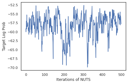
我們從 dist 取樣以產生 MCMC 的初始狀態。然後,我們可以定義一個函式,該函式接受隨機金鑰和初始狀態,並從 No-U-Turn-Sampler (NUTS) 產生 500 個樣本。請注意,我們可以使用 JAX 轉換 (例如 jit) 來編譯使用 XLA 的 NUTS 取樣器。
init_key, sample_key = random.split(random.PRNGKey(0))
init_params = tuple(dist.sample(seed=init_key)[:-1])

@jit
def run_chain(key, state):
  kernel = tfp.mcmc.NoUTurnSampler(target_log_prob, 1e-3)
  return tfp.mcmc.sample_chain(500,
      current_state=state,
      kernel=kernel,
      trace_fn=lambda _, results: results.target_log_prob,
      num_burnin_steps=500,
      seed=key)

states, log_probs = run_chain(sample_key, init_params)
plt.figure()
plt.plot(log_probs)
plt.ylabel('Target Log Prob')
plt.xlabel('Iterations of NUTS')
plt.show()
讓我們使用我們的樣本執行貝氏模型平均 (BMA),方法是平均每組權重的預測機率。
首先,讓我們撰寫一個函式,針對給定的一組參數,產生每個類別的機率。我們可以使用 dist.sample_distributions 來取得模型中的最終分佈。
def classifier_probs(params):
  dists, _ = dist.sample_distributions(seed=random.PRNGKey(0),
                                       value=params + (None,))
  return dists[-1].distribution.probs_parameter()
我們可以對樣本集 vmap(classifier_probs),以取得每個樣本的預測類別機率。然後,我們計算每個樣本的平均準確度,以及貝氏模型平均的準確度。
all_probs = jit(vmap(classifier_probs))(states)
print('Average accuracy:', jnp.mean(all_probs.argmax(axis=-1) == labels))
print('BMA accuracy:', jnp.mean(all_probs.mean(axis=0).argmax(axis=-1) == labels))
Average accuracy: 0.96952
BMA accuracy: 0.97999996
看起來 BMA 將我們的錯誤率降低了將近三分之一!
基本原理
JAX 上的 TFP 具有與 TF 相同的 API,其中 JAX 上的 TFP 接受 JAX 對應物,而不是接受 tf.Tensor 等 TF 物件。例如,先前使用 tf.Tensor 作為輸入的任何位置,API 現在都預期為 JAX DeviceArray。TFP 方法會傳回 DeviceArray,而不是傳回 tf.Tensor。JAX 上的 TFP 也適用於 JAX 物件的巢狀結構,例如 DeviceArray 的清單或字典。
分佈
JAX 支援大多數 TFP 的分佈,其語意與 TF 對應物非常相似。它們也註冊為 JAX Pytrees,因此它們可以是 JAX 轉換函式的輸入和輸出。
基本分佈
分佈的 log_prob 方法運作方式相同。
dist = tfd.Normal(0., 1.)
print(dist.log_prob(0.))
-0.9189385
從分佈取樣需要明確傳入 PRNGKey (或整數清單) 作為 seed 關鍵字引數。未能明確傳入種子將會擲回錯誤。
tfd.Normal(0., 1.).sample(seed=random.PRNGKey(0))
DeviceArray(-0.20584226, dtype=float32)
分佈的形狀語意在 JAX 中保持不變,其中分佈將各自具有 event_shape 和 batch_shape,而繪製許多樣本將會新增額外的 sample_shape 維度。
例如,具有向量參數的 tfd.MultivariateNormalDiag 將具有向量事件形狀和空批次形狀。
dist = tfd.MultivariateNormalDiag(
    loc=jnp.zeros(5),
    scale_diag=jnp.ones(5)
)
print('Event shape:', dist.event_shape)
print('Batch shape:', dist.batch_shape)
Event shape: (5,)
Batch shape: ()
另一方面,以向量參數化的 tfd.Normal 將具有純量事件形狀和向量批次形狀。
dist = tfd.Normal(
    loc=jnp.ones(5),
    scale=jnp.ones(5),
)
print('Event shape:', dist.event_shape)
print('Batch shape:', dist.batch_shape)
Event shape: ()
Batch shape: (5,)
取得樣本 log_prob 的語意在 JAX 中也以相同方式運作。
dist =  tfd.Normal(jnp.zeros(5), jnp.ones(5))
s = dist.sample(sample_shape=(10, 2), seed=random.PRNGKey(0))
print(dist.log_prob(s).shape)

dist =  tfd.Independent(tfd.Normal(jnp.zeros(5), jnp.ones(5)), 1)
s = dist.sample(sample_shape=(10, 2), seed=random.PRNGKey(0))
print(dist.log_prob(s).shape)
(10, 2, 5)
(10, 2)
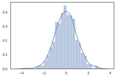
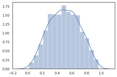
由於 JAX DeviceArray 與 NumPy 和 Matplotlib 等程式庫相容,因此我們可以將樣本直接饋送到繪圖函式中。
sns.distplot(tfd.Normal(0., 1.).sample(1000, seed=random.PRNGKey(0)))
plt.show()
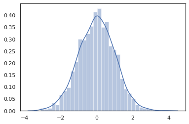
Distribution 方法與 JAX 轉換相容。
sns.distplot(jit(vmap(lambda key: tfd.Normal(0., 1.).sample(seed=key)))(
    random.split(random.PRNGKey(0), 2000)))
plt.show()
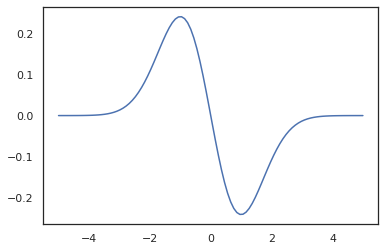
x = jnp.linspace(-5., 5., 100)
plt.plot(x, jit(vmap(grad(tfd.Normal(0., 1.).prob)))(x))
plt.show()
由於 TFP 分佈已註冊為 JAX pytree 節點,因此我們可以撰寫以分佈作為輸入或輸出的函式,並使用 jit 轉換它們,但它們尚不支援作為 vmap 函式的引數。
@jit
def random_distribution(key):
  loc_key, scale_key = random.split(key)
  loc, log_scale = random.normal(loc_key), random.normal(scale_key)
  return tfd.Normal(loc, jnp.exp(log_scale))
random_dist = random_distribution(random.PRNGKey(0))
print(random_dist.mean(), random_dist.variance())
0.14389051 0.081832744
轉換分佈
轉換分佈,即樣本透過 Bijector 傳遞的分佈,也可以立即使用 (bijector 也適用!請參閱下方)。
dist = tfd.TransformedDistribution(
    tfd.Normal(0., 1.),
    tfb.Sigmoid()
)
sns.distplot(dist.sample(1000, seed=random.PRNGKey(0)))
plt.show()
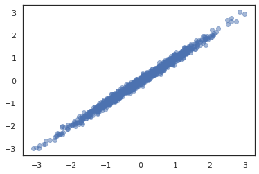
聯合分佈
TFP 提供 JointDistribution,以啟用將元件分佈組合成多個隨機變數的單一分佈。目前,TFP 提供三種核心變體 (JointDistributionSequential、JointDistributionNamed 和 JointDistributionCoroutine),所有這些變體都在 JAX 中受到支援。AutoBatched 變體也全部受到支援。
dist = tfd.JointDistributionSequential([
  tfd.Normal(0., 1.),
  lambda x: tfd.Normal(x, 1e-1)
])
plt.scatter(*dist.sample(1000, seed=random.PRNGKey(0)), alpha=0.5)
plt.show()
joint = tfd.JointDistributionNamed(dict(
    e=             tfd.Exponential(rate=1.),
    n=             tfd.Normal(loc=0., scale=2.),
    m=lambda n, e: tfd.Normal(loc=n, scale=e),
    x=lambda    m: tfd.Sample(tfd.Bernoulli(logits=m), 12),
))
joint.sample(seed=random.PRNGKey(0))
{'e': DeviceArray(3.376818, dtype=float32),
 'm': DeviceArray(2.5449684, dtype=float32),
 'n': DeviceArray(-0.6027825, dtype=float32),
 'x': DeviceArray([1, 1, 1, 1, 1, 1, 1, 1, 1, 1, 1, 1], dtype=int32)}
Root = tfd.JointDistributionCoroutine.Root
def model():
  e = yield Root(tfd.Exponential(rate=1.))
  n = yield Root(tfd.Normal(loc=0, scale=2.))
  m = yield tfd.Normal(loc=n, scale=e)
  x = yield tfd.Sample(tfd.Bernoulli(logits=m), 12)

joint = tfd.JointDistributionCoroutine(model)

joint.sample(seed=random.PRNGKey(0))
StructTuple(var0=DeviceArray(0.17315261, dtype=float32), var1=DeviceArray(-3.290489, dtype=float32), var2=DeviceArray(-3.1949058, dtype=float32), var3=DeviceArray([0, 0, 0, 0, 0, 0, 0, 0, 0, 0, 0, 0], dtype=int32))
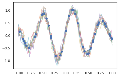
其他分佈
高斯過程在 JAX 模式下也適用!
k1, k2, k3 = random.split(random.PRNGKey(0), 3)
observation_noise_variance = 0.01
f = lambda x: jnp.sin(10*x[..., 0]) * jnp.exp(-x[..., 0]**2)
observation_index_points = random.uniform(
    k1, [50], minval=-1.,maxval= 1.)[..., jnp.newaxis]
observations = f(observation_index_points) + tfd.Normal(
    loc=0., scale=jnp.sqrt(observation_noise_variance)).sample(seed=k2)

index_points = jnp.linspace(-1., 1., 100)[..., jnp.newaxis]

kernel = tfpk.ExponentiatedQuadratic(length_scale=0.1)

gprm = tfd.GaussianProcessRegressionModel(
    kernel=kernel,
    index_points=index_points,
    observation_index_points=observation_index_points,
    observations=observations,
    observation_noise_variance=observation_noise_variance)

samples = gprm.sample(10, seed=k3)
for i in range(10):
  plt.plot(index_points, samples[i], alpha=0.5)
plt.plot(observation_index_points, observations, marker='o', linestyle='')
plt.show()
隱藏式馬可夫模型也受到支援。
initial_distribution = tfd.Categorical(probs=[0.8, 0.2])
transition_distribution = tfd.Categorical(probs=[[0.7, 0.3],
                                                 [0.2, 0.8]])

observation_distribution = tfd.Normal(loc=[0., 15.], scale=[5., 10.])

model = tfd.HiddenMarkovModel(
    initial_distribution=initial_distribution,
    transition_distribution=transition_distribution,
    observation_distribution=observation_distribution,
    num_steps=7)

print(model.mean())
print(model.log_prob(jnp.zeros(7)))
print(model.sample(seed=random.PRNGKey(0)))
[3.       6.       7.5      8.249999 8.625001 8.812501 8.90625 ]
/usr/local/lib/python3.6/dist-packages/tensorflow_probability/substrates/jax/distributions/hidden_markov_model.py:483: UserWarning: HiddenMarkovModel.log_prob in TFP versions < 0.12.0 had a bug in which the transition model was applied prior to the initial step. This bug has been fixed. You may observe a slight change in behavior.
  'HiddenMarkovModel.log_prob in TFP versions < 0.12.0 had a bug '
-19.855635
[ 1.3641367  0.505798   1.3626463  3.6541772  2.272286  15.10309
 22.794212 ]
由於嚴格依賴 TensorFlow 或 XLA 不相容性,因此目前不支援少數分佈 (例如 PixelCNN)。
Bijector
JAX 今天支援大多數 TFP 的 bijector!
tfb.Exp().inverse(1.)
DeviceArray(0., dtype=float32)
bij = tfb.Shift(1.)(tfb.Scale(3.))
print(bij.forward(jnp.ones(5)))
print(bij.inverse(jnp.ones(5)))
[4. 4. 4. 4. 4.]
[0. 0. 0. 0. 0.]
b = tfb.FillScaleTriL(diag_bijector=tfb.Exp(), diag_shift=None)
print(b.forward(x=[0., 0., 0.]))
print(b.inverse(y=[[1., 0], [.5, 2]]))
[[1. 0.]
 [0. 1.]]
[0.6931472 0.5       0.       ]
b = tfb.Chain([tfb.Exp(), tfb.Softplus()])
# or:
# b = tfb.Exp()(tfb.Softplus())
print(b.forward(-jnp.ones(5)))
[1.3678794 1.3678794 1.3678794 1.3678794 1.3678794]
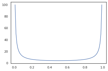
Bijector 與 JAX 轉換相容,例如 jit、grad 和 vmap。
jit(vmap(tfb.Exp().inverse))(jnp.arange(4.))
DeviceArray([ -inf, 0. , 0.6931472, 1.0986123], dtype=float32)
x = jnp.linspace(0., 1., 100)
plt.plot(x, jit(grad(lambda x: vmap(tfb.Sigmoid().inverse)(x).sum()))(x))
plt.show()
某些 bijector (例如 RealNVP 和 FFJORD) 尚不受支援。
MCMC
我們也已將 tfp.mcmc 移植到 JAX,因此我們可以在 JAX 中執行 Hamiltonian Monte Carlo (HMC) 和 No-U-Turn-Sampler (NUTS) 等演算法。
target_log_prob = tfd.MultivariateNormalDiag(jnp.zeros(2), jnp.ones(2)).log_prob
與 TF 上的 TFP 不同,我們需要使用 seed 關鍵字引數將 PRNGKey 傳遞到 sample_chain 中。
def run_chain(key, state):
kernel = tfp.mcmc.NoUTurnSampler(target_log_prob, 1e-1)
return tfp.mcmc.sample_chain(1000,
current_state=state,
kernel=kernel,
trace_fn=lambda _, results: results.target_log_prob,
seed=key)
states, log_probs = jit(run_chain)(random.PRNGKey(0), jnp.zeros(2))
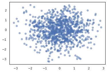
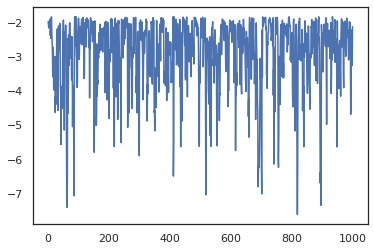
plt.figure()
plt.scatter(*states.T, alpha=0.5)
plt.figure()
plt.plot(log_probs)
plt.show()
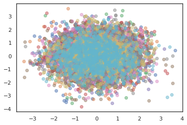
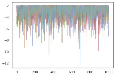
若要執行多個鏈,我們可以將一批狀態傳遞到 sample_chain 中,或使用 vmap (雖然我們尚未探索這兩種方法之間的效能差異)。
states, log_probs = jit(run_chain)(random.PRNGKey(0), jnp.zeros([10, 2]))
plt.figure()
for i in range(10):
  plt.scatter(*states[:, i].T, alpha=0.5)
plt.figure()
for i in range(10):
  plt.plot(log_probs[:, i], alpha=0.5)
plt.show()
最佳化工具
JAX 上的 TFP 支援一些重要的最佳化工具,例如 BFGS 和 L-BFGS。讓我們設定一個簡單的縮放二次損失函數。
minimum = jnp.array([1.0, 1.0])  # The center of the quadratic bowl.
scales = jnp.array([2.0, 3.0])  # The scales along the two axes.

# The objective function and the gradient.
def quadratic_loss(x):
  return jnp.sum(scales * jnp.square(x - minimum))

start = jnp.array([0.6, 0.8])  # Starting point for the search.
BFGS 可以找到此損失的最小值。
optim_results = tfp.optimizer.bfgs_minimize(
    value_and_grad(quadratic_loss), initial_position=start, tolerance=1e-8)

# Check that the search converged
assert(optim_results.converged)
# Check that the argmin is close to the actual value.
np.testing.assert_allclose(optim_results.position, minimum)
# Print out the total number of function evaluations it took. Should be 5.
print("Function evaluations: %d" % optim_results.num_objective_evaluations)
Function evaluations: 5
L-BFGS 也可以。
optim_results = tfp.optimizer.lbfgs_minimize(
    value_and_grad(quadratic_loss), initial_position=start, tolerance=1e-8)

# Check that the search converged
assert(optim_results.converged)
# Check that the argmin is close to the actual value.
np.testing.assert_allclose(optim_results.position, minimum)
# Print out the total number of function evaluations it took. Should be 5.
print("Function evaluations: %d" % optim_results.num_objective_evaluations)
Function evaluations: 5
若要 vmap L-BFGS,讓我們設定一個函式,該函式針對單一起點最佳化損失。
def optimize_single(start):
  return tfp.optimizer.lbfgs_minimize(
      value_and_grad(quadratic_loss), initial_position=start, tolerance=1e-8)

all_results = jit(vmap(optimize_single))(
    random.normal(random.PRNGKey(0), (10, 2)))
assert all(all_results.converged)
for i in range(10):
  np.testing.assert_allclose(optim_results.position[i], minimum)
print("Function evaluations: %s" % all_results.num_objective_evaluations)
Function evaluations: [6 6 9 6 6 8 6 8 5 9]
注意事項
TF 和 JAX 之間存在一些基本差異,某些 TFP 行為在兩個基底之間會有所不同,而且並非所有功能都受到支援。例如:
- JAX 上的 TFP 不支援任何類似
tf.Variable的項目,因為 JAX 中不存在類似項目。這也表示tfp.util.TransformedVariable等公用程式也不受支援。 - 由於
tfp.layers依賴 Keras 和tf.Variable,因此後端尚不支援tfp.layers。 - 由於
tfp.math.minimize依賴tf.Variable,因此 TFP on JAX 無法運作tfp.math.minimize。 - 使用 JAX 上的 TFP 時,張量形狀一律為具體的整數值,而且絕不會像 TF 上的 TFP 那樣未知/動態。
- 虛擬隨機性在 TF 和 JAX 中的處理方式不同 (請參閱附錄)。
tfp.experimental中的程式庫不保證存在於 JAX 基底中。- TF 和 JAX 之間的 Dtype 升級規則不同。JAX 上的 TFP 會嘗試在內部遵循 TF 的 dtype 語意,以保持一致性。
- Bijector 尚未註冊為 JAX pytree。
若要查看 JAX 上的 TFP 支援的完整清單,請參閱 API 文件。
結論
我們已將許多 TFP 的功能移植到 JAX,並很高興看到大家將建構什麼。某些功能尚不受支援;如果您發現我們遺漏了對您重要的項目 (或您發現錯誤!),請與我們聯絡 -- 您可以傳送電子郵件至 tfprobability@tensorflow.org,或在 我們的 Github 存放區上提出問題。
附錄:JAX 中的虛擬隨機性
JAX 的虛擬隨機數字產生 (PRNG) 模型是無狀態的。與有狀態模型不同,沒有在每次隨機繪製後演變的可變全域狀態。在 JAX 的模型中,我們從 PRNG 金鑰開始,其作用類似於一對 32 位元整數。我們可以使用 jax.random.PRNGKey 建構這些金鑰。
key = random.PRNGKey(0)  # Creates a key with value [0, 0]
print(key)
[0 0]
JAX 中的隨機函式會使用金鑰來確定性產生隨機變數,表示它們不應再次使用。例如,我們可以使用 key 取樣常態分佈值,但我們不應在其他地方再次使用 key。此外,將相同的值傳遞到 random.normal 將會產生相同的值。
print(random.normal(key))
-0.20584226
那麼,我們如何從單一金鑰中繪製多個樣本?答案是金鑰分割。基本概念是我們可以將 PRNGKey 分割成多個,而每個新金鑰都可以視為獨立的隨機性來源。
key1, key2 = random.split(key, num=2)
print(key1, key2)
[4146024105 967050713] [2718843009 1272950319]
金鑰分割是確定性的,但具有混沌性,因此現在每個新金鑰都可以用來繪製不同的隨機樣本。
print(random.normal(key1), random.normal(key2))
0.14389051 -1.2515389
如需 JAX 確定性金鑰分割模型的詳細資訊,請參閱本指南。