在 TensorFlow.org 上檢視

在 Google Colab 中執行

在 GitHub 上檢視原始碼

下載筆記本

我撰寫這個筆記本作為案例研究，以學習 TensorFlow Probability。我選擇解決的問題是估計 2 維平均值為 0 的高斯隨機變數樣本的共變異數矩陣。這個問題有幾個優點：

• 如果我們對共變異數使用反向 Wishart 先驗 (常見方法)，此問題會有解析解，因此我們可以檢查結果。
• 此問題牽涉到對受限參數進行取樣，這增加了一些有趣的複雜性。
• 最直接的解決方案不是最快的解決方案，因此還有一些最佳化工作要做。

我決定在我進行時寫下我的經驗。我花了一段時間才理解 TFP 的更精細之處，因此這個筆記本從相當簡單的內容開始，然後逐步深入到更複雜的 TFP 功能。我一路遇到了許多問題，並且嘗試記錄下協助我找出問題的過程，以及我最終找到的解決方法。我嘗試包含大量細節 (包括大量測試，以確保個別步驟正確無誤)。

為何要學習 TensorFlow Probability？

我發現 TensorFlow Probability 對我的專案很有吸引力，原因如下：

• TensorFlow Probability 讓您可以在筆記本中以互動方式建立原型並開發複雜的模型。您可以將程式碼分成小塊，以便以互動方式進行測試和單元測試。
• 一旦您準備好擴大規模，就可以充分利用我們已建置的所有基礎架構，讓 TensorFlow 在多部機器上的多個最佳化處理器上執行。
• 最後，雖然我真的很喜歡 Stan，但我發現它很難偵錯。您必須以獨立語言撰寫所有模型程式碼，而這種語言幾乎沒有任何工具可讓您探查程式碼、檢查中間狀態等等。

缺點是 TensorFlow Probability 比 Stan 和 PyMC3 新得多，因此文件仍在建置中，而且還有許多功能尚待建置。令人高興的是，我發現 TFP 的基礎很穩固，而且它以模組化方式設計，可讓人相當直接地擴充其功能。在這個筆記本中，除了解決案例研究之外，我還會展示一些擴充 TFP 的方法。

適用對象

我假設讀者在閱讀這個筆記本之前已具備一些重要的先備知識。您應該：

• 了解貝氏推論的基本知識。(如果您不了解，一本非常好的入門書是Statistical Rethinking)
• 熟悉 MCMC 取樣程式庫，例如 Stan / PyMC3 / BUGS
• 紮實掌握 NumPy (一本不錯的入門書是Python for Data Analysis)
• 至少略為熟悉 TensorFlow，但不一定需要專業知識。(Learning TensorFlow 不錯，但 TensorFlow 的快速發展表示大多數書籍都會有點過時。史丹佛大學的 CS20 課程也不錯。)

初次嘗試

這是我第一次嘗試解決這個問題。劇透：我的解決方案無效，而且需要多次嘗試才能正確！雖然這個過程需要一段時間，但以下每次嘗試都對學習 TFP 的新部分很有幫助。

注意事項：TFP 目前未實作反向 Wishart 分配 (我們會在最後看到如何自行推出反向 Wishart)，因此我會將問題變更為使用 Wishart 先驗估計精確度矩陣的問題。

import collections
import math
import os
import time

import numpy as np
import pandas as pd
import scipy
import scipy.stats
import matplotlib.pyplot as plt

import tensorflow.compat.v2 as tf
tf.enable_v2_behavior()
import tensorflow_probability as tfp
tfd = tfp.distributions
tfb = tfp.bijectors

步驟 1：將觀測值彙整在一起

我這裡的資料都是合成的，因此看起來會比真實世界的範例更整潔。但是，沒有理由您不能產生一些自己的合成資料。

提示：一旦您決定模型的形式，就可以選擇一些參數值，並使用您選擇的模型來產生一些合成資料。作為實作的健全性檢查，您可以驗證您的估計是否包含您選擇的參數的真實值。為了加快偵錯/測試週期，您可以考慮模型的簡化版本 (例如，使用較少的維度或較少的樣本)。

提示： 最容易將您的觀測值當作 NumPy 陣列來使用。一個重要的注意事項是，NumPy 預設使用 float64，而 TensorFlow 預設使用 float32。

一般而言，TensorFlow 運算希望所有引數都具有相同的類型，而且您必須執行明確的資料轉換才能變更類型。如果您使用 float64 觀測值，則需要加入許多轉換運算。相反地，NumPy 會自動處理轉換。因此，將您的 Numpy 資料轉換為 float32 比強迫 TensorFlow 使用 float64 容易得多。

選擇一些參數值

# We're assuming 2-D data with a known true mean of (0, 0)
true_mean = np.zeros([2], dtype=np.float32)
# We'll make the 2 coordinates correlated
true_cor = np.array([[1.0, 0.9], [0.9, 1.0]], dtype=np.float32)
# And we'll give the 2 coordinates different variances
true_var = np.array([4.0, 1.0], dtype=np.float32)
# Combine the variances and correlations into a covariance matrix
true_cov = np.expand_dims(np.sqrt(true_var), axis=1).dot(
    np.expand_dims(np.sqrt(true_var), axis=1).T) * true_cor
# We'll be working with precision matrices, so we'll go ahead and compute the
# true precision matrix here
true_precision = np.linalg.inv(true_cov)

# Here's our resulting covariance matrix
print(true_cov)
# Verify that it's positive definite, since np.random.multivariate_normal
# complains about it not being positive definite for some reason.
# (Note that I'll be including a lot of sanity checking code in this notebook -
# it's a *huge* help for debugging)
print('eigenvalues: ', np.linalg.eigvals(true_cov))

[[4.  1.8]
 [1.8 1. ]]
eigenvalues:  [4.843075   0.15692513]

產生一些合成觀測值

請注意，TensorFlow Probability 使用的慣例是，資料的初始維度代表樣本索引，而資料的最終維度代表樣本的維度。

這裡我們想要 100 個樣本，每個樣本都是長度為 2 的向量。我們將產生一個形狀為 (100, 2) 的陣列 my_data。my_data[i, :] 是第 \(i\) 個樣本，它是一個長度為 2 的向量。

(請記住讓 my_data 具有 float32 類型！)

# Set the seed so the results are reproducible.
np.random.seed(123)

# Now generate some observations of our random variable.
# (Note that I'm suppressing a bunch of spurious about the covariance matrix
# not being positive semidefinite via check_valid='ignore' because it really is
# positive definite!)
my_data = np.random.multivariate_normal(
    mean=true_mean, cov=true_cov, size=100,
    check_valid='ignore').astype(np.float32)

my_data.shape

(100, 2)

健全性檢查觀測值

一個潛在的錯誤來源是搞亂您的合成資料！讓我們做一些簡單的檢查。

# Do a scatter plot of the observations to make sure they look like what we
# expect (higher variance on the x-axis, y values strongly correlated with x)
plt.scatter(my_data[:, 0], my_data[:, 1], alpha=0.75)
plt.show()

print('mean of observations:', np.mean(my_data, axis=0))
print('true mean:', true_mean)

mean of observations: [-0.24009615 -0.16638893]
true mean: [0. 0.]

print('covariance of observations:\n', np.cov(my_data, rowvar=False))
print('true covariance:\n', true_cov)

covariance of observations:
 [[3.95307734 1.68718486]
 [1.68718486 0.94910269]]
true covariance:
 [[4.  1.8]
 [1.8 1. ]]

好的，我們的樣本看起來合理。下一步。

步驟 2：在 NumPy 中實作概似函數

我們需要撰寫以在 TF Probability 中執行 MCMC 取樣的主要內容是對數概似函數。一般而言，撰寫 TF 比 NumPy 更棘手，因此我發現先在 NumPy 中進行初始實作很有幫助。我將把概似函數分成 2 個部分：資料概似函數 (對應於 \(P(data | parameters)\)) 和先驗概似函數 (對應於 \(P(parameters)\))。

請注意，這些 NumPy 函數不必經過超級最佳化/向量化，因為目標只是產生一些值以進行測試。正確性是關鍵考量！

首先，我們將實作資料對數概似部分。這非常簡單。要記住的一件事是，我們將使用精確度矩陣，因此我們將相應地參數化。

def log_lik_data_numpy(precision, data):
  # np.linalg.inv is a really inefficient way to get the covariance matrix, but
  # remember we don't care about speed here
  cov = np.linalg.inv(precision)
  rv = scipy.stats.multivariate_normal(true_mean, cov)
  return np.sum(rv.logpdf(data))

# test case: compute the log likelihood of the data given the true parameters
log_lik_data_numpy(true_precision, my_data)

-280.81822950593767

我們將對精確度矩陣使用 Wishart 先驗，因為後驗有解析解 (請參閱 維基百科方便的共軛先驗表)。

Wishart 分配 有 2 個參數：

• 自由度數 (在維基百科中標記為 \(\nu\))
• 比例矩陣 (在維基百科中標記為 \(V\))

具有參數 \(\nu, V\) 的 Wishart 分配的平均值為 \(E[W] = \nu V\)，而變異數為 \(\text{Var}(W_{ij}) = \nu(v_{ij}^2+v_{ii}v_{jj})\)

一些有用的直覺：您可以透過從具有平均值 0 和共變異數 \(V\) 的多變數常態隨機變數中產生 \(\nu\) 個獨立繪圖 \(x_1 \ldots x_{\nu}\)，然後形成總和 \(W = \sum_{i=1}^{\nu} x_i x_i^T\)，來產生 Wishart 樣本。

如果您透過將 Wishart 樣本除以 \(\nu\) 來重新調整其比例，您會得到 \(x_i\) 的樣本共變異數矩陣。隨著 \(\nu\) 增加，此樣本共變異數矩陣應該趨向於 \(V\)。當 \(\nu\) 很小時，樣本共變異數矩陣中有很多變異，因此 \(\nu\) 的小值對應於較弱的先驗，而 \(\nu\) 的大值對應於較強的先驗。請注意，\(\nu\) 必須至少與您取樣的空間的維度一樣大，否則您將產生奇異矩陣。

我們將使用 \(\nu = 3\)，因此我們有一個弱先驗，而且我們將取 \(V = \frac{1}{\nu} I\)，這會將我們的共變異數估計值拉向單位矩陣 (回想一下，平均值為 \(\nu V\))。

PRIOR_DF = 3
PRIOR_SCALE = np.eye(2, dtype=np.float32) / PRIOR_DF

def log_lik_prior_numpy(precision):
  rv = scipy.stats.wishart(df=PRIOR_DF, scale=PRIOR_SCALE)
  return rv.logpdf(precision)

# test case: compute the prior for the true parameters
log_lik_prior_numpy(true_precision)

-9.103606346649766

Wishart 分配是估計具有已知平均值 \(\mu\) 的多變數常態的精確度矩陣的共軛先驗。

假設先驗 Wishart 參數為 \(\nu, V\)，並且我們有 \(n\) 個多變數常態觀測值 \(x_1, \ldots, x_n\)。後驗參數為 \(n + \nu, \left(V^{-1} + \sum_{i=1}^n (x_i-\mu)(x_i-\mu)^T \right)^{-1}\)。

n = my_data.shape[0]
nu_prior = PRIOR_DF
v_prior = PRIOR_SCALE
nu_posterior = nu_prior + n
v_posterior = np.linalg.inv(np.linalg.inv(v_prior) + my_data.T.dot(my_data))
posterior_mean = nu_posterior * v_posterior
v_post_diag = np.expand_dims(np.diag(v_posterior), axis=1)
posterior_sd = np.sqrt(nu_posterior *
                       (v_posterior ** 2.0 + v_post_diag.dot(v_post_diag.T)))

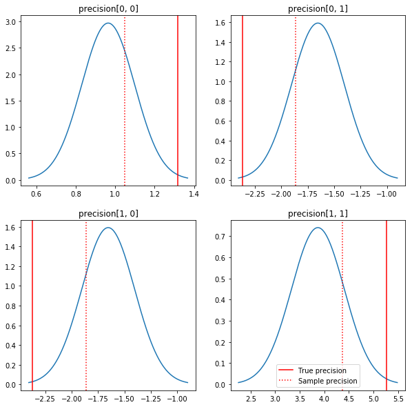
後驗和真實值的快速繪圖。請注意，後驗接近樣本後驗，但略微向單位矩陣收縮。另請注意，真實值與後驗的眾數相差甚遠 - 大概是因為先驗與我們的資料不太匹配。在真實問題中，我們可能會使用縮放的反向 Wishart 先驗來獲得更好的結果 (例如，請參閱 Andrew Gelman 關於此主題的 評論)，但這樣我們就不會有很好的解析後驗。

sample_precision = np.linalg.inv(np.cov(my_data, rowvar=False, bias=False))
fig, axes = plt.subplots(2, 2)
fig.set_size_inches(10, 10)
for i in range(2):
  for j in range(2):
    ax = axes[i, j]
    loc = posterior_mean[i, j]
    scale = posterior_sd[i, j]
    xmin = loc - 3.0 * scale
    xmax = loc + 3.0 * scale
    x = np.linspace(xmin, xmax, 1000)
    y = scipy.stats.norm.pdf(x, loc=loc, scale=scale)
    ax.plot(x, y)
    ax.axvline(true_precision[i, j], color='red', label='True precision')
    ax.axvline(sample_precision[i, j], color='red', linestyle=':', label='Sample precision')
    ax.set_title('precision[%d, %d]' % (i, j))
plt.legend()
plt.show()

步驟 3：在 TensorFlow 中實作概似函數

劇透：我們的第一次嘗試不會成功；我們將在下面討論原因。

提示：在開發概似函數時，請使用 TensorFlow eager 模式。Eager 模式使 TF 的行為更像 NumPy - 所有內容都會立即執行，因此您可以以互動方式進行偵錯，而不必使用 Session.run()。請參閱此處的注意事項。

初步：分配類別

TFP 有一系列分配類別，我們將使用它們來產生對數機率。一個需要注意的事項是，這些類別處理的是樣本張量，而不僅僅是單個樣本 - 這允許向量化和相關的加速。

分配可以透過 2 種不同的方式處理樣本張量。最簡單的方法是用一個具體的範例來說明這 2 種方式，該範例涉及具有單一純量參數的分配。我將使用 Poisson 分配，它具有 rate 參數。

• 如果我們建立一個 rate 參數具有單一值的 Poisson，則呼叫其 sample() 方法會傳回單一值。此值稱為事件，在這種情況下，事件都是純量。
• 如果我們建立一個 rate 參數具有值張量的 Poisson，則呼叫其 sample() 方法現在會傳回多個值，每個值對應於 rate 張量中的一個值。此物件充當獨立 Poisson 的集合，每個 Poisson 都有自己的 rate，並且對 sample() 的呼叫傳回的每個值都對應於其中一個 Poisson。這個獨立但非恆等分配事件的集合稱為批次。
• sample() 方法採用 sample_shape 參數，預設值為空元組。為 sample_shape 傳遞非空值會導致 sample 傳回多個批次。這個批次集合稱為 樣本。

分配的 log_prob() 方法以與 sample() 產生資料的方式平行的方式來消耗資料。log_prob() 傳回樣本的機率，即多個獨立的事件批次的機率。

• 如果我們的 Poisson 物件是以純量 rate 建立的，則每個批次都是純量，而且如果我們傳入樣本張量，我們將得到相同大小的對數機率張量。
• 如果我們的 Poisson 物件是以形狀為 T 的 rate 值張量建立的，則每個批次都是形狀為 T 的張量。如果我們傳入形狀為 D, T 的樣本張量，我們將得到形狀為 D, T 的對數機率張量。

以下是一些範例，說明這些情況。請參閱 此筆記本，以取得關於事件、批次和形狀的更詳細教學課程。

# case 1: get log probabilities for a vector of iid draws from a single
# normal distribution
norm1 = tfd.Normal(loc=0., scale=1.)
probs1 = norm1.log_prob(tf.constant([1., 0.5, 0.]))

# case 2: get log probabilities for a vector of independent draws from
# multiple normal distributions with different parameters.  Note the vector
# values for loc and scale in the Normal constructor.
norm2 = tfd.Normal(loc=[0., 2., 4.], scale=[1., 1., 1.])
probs2 = norm2.log_prob(tf.constant([1., 0.5, 0.]))

print('iid draws from a single normal:', probs1.numpy())
print('draws from a batch of normals:', probs2.numpy())

iid draws from a single normal: [-1.4189385 -1.0439385 -0.9189385]
draws from a batch of normals: [-1.4189385 -2.0439386 -8.918939 ]

資料對數概似

首先，我們將實作資料對數概似函數。

VALIDATE_ARGS = True
ALLOW_NAN_STATS = False

與 NumPy 案例的一個主要區別在於，我們的 TensorFlow 概似函數需要處理精確度矩陣的向量，而不僅僅是單個矩陣。當我們從多個鏈取樣時，將會使用參數向量。

我們將建立一個分配物件，該物件可處理一批精確度矩陣 (即每個鏈一個矩陣)。

在計算資料的對數機率時，我們需要以與參數相同的方式複製資料，以便每個批次變數都有一個副本。複製資料的形狀需要如下：

[樣本形狀、批次形狀、事件形狀]

在我們的案例中，事件形狀為 2 (因為我們正在處理 2 維高斯)。樣本形狀為 100，因為我們有 100 個樣本。批次形狀將只是我們正在處理的精確度矩陣的數量。每次呼叫概似函數時都複製資料是很浪費的，因此我們將提前複製資料並傳入複製版本。

請注意，這是一種效率低下的實作：相對於我們將在最後的最佳化章節中討論的一些替代方案，MultivariateNormalFullCovariance 的成本很高。

def log_lik_data(precisions, replicated_data):
  n = tf.shape(precisions)[0]  # number of precision matrices
  # We're estimating a precision matrix; we have to invert to get log
  # probabilities.  Cholesky inversion should be relatively efficient,
  # but as we'll see later, it's even better if we can avoid doing the Cholesky
  # decomposition altogether.
  precisions_cholesky = tf.linalg.cholesky(precisions)
  covariances = tf.linalg.cholesky_solve(
      precisions_cholesky, tf.linalg.eye(2, batch_shape=[n]))
  rv_data = tfd.MultivariateNormalFullCovariance(
      loc=tf.zeros([n, 2]),
      covariance_matrix=covariances,
      validate_args=VALIDATE_ARGS,
      allow_nan_stats=ALLOW_NAN_STATS)

  return tf.reduce_sum(rv_data.log_prob(replicated_data), axis=0)

# For our test, we'll use a tensor of 2 precision matrices.
# We'll need to replicate our data for the likelihood function.
# Remember, TFP wants the data to be structured so that the sample dimensions
# are first (100 here), then the batch dimensions (2 here because we have 2
# precision matrices), then the event dimensions (2 because we have 2-D
# Gaussian data).  We'll need to add a middle dimension for the batch using
# expand_dims, and then we'll need to create 2 replicates in this new dimension
# using tile.
n = 2
replicated_data = np.tile(np.expand_dims(my_data, axis=1), reps=[1, 2, 1])
print(replicated_data.shape)

(100, 2, 2)

提示： 我發現非常有幫助的一件事是撰寫 TensorFlow 函數的小型健全性檢查。在 TF 中搞亂向量化真的很容易，因此備妥更簡單的 NumPy 函數是驗證 TF 輸出的絕佳方法。將這些視為小型單元測試。

# check against the numpy implementation
precisions = np.stack([np.eye(2, dtype=np.float32), true_precision])
n = precisions.shape[0]
lik_tf = log_lik_data(precisions, replicated_data=replicated_data).numpy()

for i in range(n):
  print(i)
  print('numpy:', log_lik_data_numpy(precisions[i], my_data))
  print('tensorflow:', lik_tf[i])

0
numpy: -430.71218815801365
tensorflow: -430.71207
1
numpy: -280.81822950593767
tensorflow: -280.8182

先驗對數概似

先驗更簡單，因為我們不必擔心資料複製。

@tf.function(autograph=False)
def log_lik_prior(precisions):
  rv_precision = tfd.WishartTriL(
      df=PRIOR_DF,
      scale_tril=tf.linalg.cholesky(PRIOR_SCALE),
      validate_args=VALIDATE_ARGS,
      allow_nan_stats=ALLOW_NAN_STATS)
  return rv_precision.log_prob(precisions)

# check against the numpy implementation
precisions = np.stack([np.eye(2, dtype=np.float32), true_precision])
n = precisions.shape[0]
lik_tf = log_lik_prior(precisions).numpy()

for i in range(n):
  print(i)
  print('numpy:', log_lik_prior_numpy(precisions[i]))
  print('tensorflow:', lik_tf[i])

0
numpy: -2.2351873809649625
tensorflow: -2.2351875
1
numpy: -9.103606346649766
tensorflow: -9.103608

建構聯合對數概似函數

上面的資料對數概似函數取決於我們的觀測值，但取樣器不會有這些觀測值。我們可以透過使用 [閉包](https://en.wikipedia.org/wiki/Closure_(computer_programming)) 來消除依賴性，而無需使用全域變數。閉包涉及一個外部函數，該函數建構一個包含內部函數所需變數的環境。

def get_log_lik(data, n_chains=1):
  # The data argument that is passed in will be available to the inner function
  # below so it doesn't have to be passed in as a parameter.
  replicated_data = np.tile(np.expand_dims(data, axis=1), reps=[1, n_chains, 1])

  @tf.function(autograph=False)
  def _log_lik(precision):
    return log_lik_data(precision, replicated_data) + log_lik_prior(precision)

  return _log_lik

步驟 4：取樣

好的，是時候取樣了！為了簡化起見，我們只使用 1 個鏈，並將單位矩陣用作起點。稍後我們將更仔細地處理。

同樣，這不會成功 - 我們會收到例外狀況。

@tf.function(autograph=False)
def sample():
  tf.random.set_seed(123)
  init_precision = tf.expand_dims(tf.eye(2), axis=0)

  # Use expand_dims because we want to pass in a tensor of starting values
  log_lik_fn = get_log_lik(my_data, n_chains=1)

  # we'll just do a few steps here
  num_results = 10
  num_burnin_steps = 10
  states = tfp.mcmc.sample_chain(
     num_results=num_results,
     num_burnin_steps=num_burnin_steps,
     current_state=[
         init_precision,
     ],
     kernel=tfp.mcmc.HamiltonianMonteCarlo(
         target_log_prob_fn=log_lik_fn,
         step_size=0.1,
         num_leapfrog_steps=3),
     trace_fn=None,
     seed=123)
  return states

try:
  states = sample()
except Exception as e:
  # shorten the giant stack trace
  lines = str(e).split('\n')
  print('\n'.join(lines[:5]+['...']+lines[-3:]))

Cholesky decomposition was not successful. The input might not be valid.
     [[{ {node mcmc_sample_chain/trace_scan/while/body/_79/smart_for_loop/while/body/_371/mh_one_step/hmc_kernel_one_step/leapfrog_integrate/while/body/_537/leapfrog_integrate_one_step/maybe_call_fn_and_grads/value_and_gradients/StatefulPartitionedCall/Cholesky} }]] [Op:__inference_sample_2849]

Function call stack:
sample
...
Function call stack:
sample

找出問題

InvalidArgumentError (請參閱上面的追蹤堆疊)：Cholesky 分解不成功。輸入可能無效。 這不是很有幫助。讓我們看看是否可以找出更多關於發生了什麼事。

• 我們將印出每個步驟的參數，以便我們可以查看失敗的值
• 我們將新增一些判斷提示，以防止特定問題。

判斷提示很棘手，因為它們是 TensorFlow 運算，而且我們必須注意確保它們被執行，並且不會從圖表中最佳化掉。如果您不熟悉 TF 判斷提示，則值得閱讀 此 TensorFlow 偵錯概觀。您可以使用 tf.control_dependencies 明確強制執行判斷提示 (請參閱以下程式碼中的註解)。

TensorFlow 的原生 Print 函數具有與判斷提示相同的行為 - 它是一種運算，而且您需要小心確保它執行。Print 在我們在筆記本中工作時會造成更多麻煩：其輸出會傳送到 stderr，而 stderr 不會顯示在儲存格中。我們將在這裡使用一個技巧：我們將透過 tf.pyfunc 建立我們自己的 TensorFlow 印出運算，而不是使用 tf.Print。與判斷提示一樣，我們必須確保我們的方法執行。

def get_log_lik_verbose(data, n_chains=1):
  # The data argument that is passed in will be available to the inner function
  # below so it doesn't have to be passed in as a parameter.
  replicated_data = np.tile(np.expand_dims(data, axis=1), reps=[1, n_chains, 1])

  def _log_lik(precisions):
    # An internal method we'll make into a TensorFlow operation via tf.py_func
    def _print_precisions(precisions):
      print('precisions:\n', precisions)
      return False  # operations must return something!
    # Turn our method into a TensorFlow operation
    print_op = tf.compat.v1.py_func(_print_precisions, [precisions], tf.bool)

    # Assertions are also operations, and some care needs to be taken to ensure
    # that they're executed
    assert_op = tf.assert_equal(
        precisions, tf.linalg.matrix_transpose(precisions),
        message='not symmetrical', summarize=4, name='symmetry_check')

    # The control_dependencies statement forces its arguments to be executed
    # before subsequent operations
    with tf.control_dependencies([print_op, assert_op]):
      return (log_lik_data(precisions, replicated_data) +
              log_lik_prior(precisions))

  return _log_lik

@tf.function(autograph=False)
def sample():
  tf.random.set_seed(123)
  init_precision = tf.eye(2)[tf.newaxis, ...]
  log_lik_fn = get_log_lik_verbose(my_data)
  # we'll just do a few steps here
  num_results = 10
  num_burnin_steps = 10
  states = tfp.mcmc.sample_chain(
      num_results=num_results,
      num_burnin_steps=num_burnin_steps,
      current_state=[
          init_precision,
      ],
      kernel=tfp.mcmc.HamiltonianMonteCarlo(
          target_log_prob_fn=log_lik_fn,
          step_size=0.1,
          num_leapfrog_steps=3),
      trace_fn=None,
      seed=123)

try:
  states = sample()
except Exception as e:
  # shorten the giant stack trace
  lines = str(e).split('\n')
  print('\n'.join(lines[:5]+['...']+lines[-3:]))

precisions:
 [[[1. 0.]
  [0. 1.]]]
precisions:
 [[[1. 0.]
  [0. 1.]]]
precisions:
 [[[ 0.24315196 -0.2761638 ]
  [-0.33882257  0.8622    ]]]
 assertion failed: [not symmetrical] [Condition x == y did not hold element-wise:] [x (leapfrog_integrate_one_step/add:0) = ] [[[0.243151963 -0.276163787][-0.338822573 0.8622]]] [y (leapfrog_integrate_one_step/maybe_call_fn_and_grads/value_and_gradients/matrix_transpose/transpose:0) = ] [[[0.243151963 -0.338822573][-0.276163787 0.8622]]]
     [[{ {node mcmc_sample_chain/trace_scan/while/body/_96/smart_for_loop/while/body/_381/mh_one_step/hmc_kernel_one_step/leapfrog_integrate/while/body/_503/leapfrog_integrate_one_step/maybe_call_fn_and_grads/value_and_gradients/symmetry_check_1/Assert/AssertGuard/else/_577/Assert} }]] [Op:__inference_sample_4837]

Function call stack:
sample
...
Function call stack:
sample

為何會失敗

取樣器嘗試的第一個新參數值是不對稱矩陣。這會導致 Cholesky 分解失敗，因為它僅針對對稱 (且正定) 矩陣定義。

這裡的問題是我們感興趣的參數是精確度矩陣，而精確度矩陣必須是實數、對稱且正定的。取樣器對此限制一無所知 (可能透過梯度除外)，因此取樣器完全有可能會提出無效值，從而導致例外狀況，尤其是當步長很大時。

對於 Hamiltonian Monte Carlo 取樣器，我們或許可以透過使用非常小的步長來解決此問題，因為梯度應該使參數遠離無效區域，但是小步長意味著收斂速度慢。對於 Metropolis-Hastings 取樣器 (它對梯度一無所知)，我們注定要失敗。

第 2 版：重新參數化為不受約束的參數

上述問題有一個直接的解決方案：我們可以重新參數化我們的模型，以便新參數不再具有這些限制。TFP 提供了一組有用的工具 - 雙射器 - 來做到這一點。

使用雙射器重新參數化

我們的精確度矩陣必須是實數且對稱的；我們想要一種沒有這些限制的替代參數化。一個起點是精確度矩陣的 Cholesky 分解。Cholesky 因子仍然受到約束 - 它們是下三角矩陣，並且它們的對角元素必須為正數。但是，如果我們取 Cholesky 因子的對角線的對數，則對數不再受限於為正數，然後如果我們將下三角部分展平為一維向量，我們就不再有下三角限制。在我們的案例中，結果將是沒有約束的長度為 3 的向量。

(Stan 手冊 有一個很棒的章節，介紹如何使用轉換來移除參數上的各種約束。)

這種重新參數化對我們的資料對數概似函數幾乎沒有影響 - 我們只需要反轉我們的轉換，以便我們取回精確度矩陣 - 但對先驗的影響更複雜。我們已指定給定精確度矩陣的機率由 Wishart 分配給出；我們的轉換矩陣的機率是多少？

回想一下，如果我們將單調函數 \(g\) 應用於一維隨機變數 \(X\)，\(Y = g(X)\)，則 \(Y\) 的密度由下式給出：

\[ f_Y(y) = | \frac{d}{dy}(g^{-1}(y)) | f_X(g^{-1}(y)) \]

\(g^{-1}\) 項的導數說明了 \(g\) 如何變更局部體積。對於更高維度的隨機變數，校正因子是 \(g^{-1}\) 的 Jacobian 行列式的絕對值 (請參閱此處)。

我們必須將反向轉換的 Jacobian 新增到我們的對數先驗概似函數中。令人高興的是，TFP 的 Bijector 類別可以為我們處理這個問題。

Bijector 類別用於表示可逆、平滑的函數，這些函數用於變更機率密度函數中的變數。雙射器都具有執行轉換的 forward() 方法、反轉轉換的 inverse() 方法，以及在我們重新參數化 pdf 時提供我們需要的 Jacobian 校正的 forward_log_det_jacobian() 和 inverse_log_det_jacobian() 方法。

TFP 提供了一系列實用的雙射函數 (bijector)，我們可以透過 Chain 運算子將它們組合起來，形成相當複雜的轉換。在我們的例子中，我們將組合以下 3 個雙射函數（鏈中的運算從右到左執行）：

1. 我們轉換的第一步是對精度矩陣執行 Cholesky 分解。雖然沒有針對此操作的 Bijector 類別，但 CholeskyOuterProduct 雙射函數會取兩個 Cholesky 因子的乘積。我們可以使用 Invert 運算子來反轉該運算。
2. 下一步是取 Cholesky 因子對角線元素的對數。我們透過 TransformDiagonal 雙射函數和 Exp 雙射函數的反函數來完成此操作。
3. 最後，我們使用 FillTriangular 雙射函數的反函數，將矩陣的下三角部分展平為向量。

# Our transform has 3 stages that we chain together via composition:
precision_to_unconstrained = tfb.Chain([
    # step 3: flatten the lower triangular portion of the matrix
    tfb.Invert(tfb.FillTriangular(validate_args=VALIDATE_ARGS)),
    # step 2: take the log of the diagonals    
    tfb.TransformDiagonal(tfb.Invert(tfb.Exp(validate_args=VALIDATE_ARGS))),
    # step 1: decompose the precision matrix into its Cholesky factors
    tfb.Invert(tfb.CholeskyOuterProduct(validate_args=VALIDATE_ARGS)),
])

# sanity checks
m = tf.constant([[1., 2.], [2., 8.]])
m_fwd = precision_to_unconstrained.forward(m)
m_inv = precision_to_unconstrained.inverse(m_fwd)

# bijectors handle tensors of values, too!
m2 = tf.stack([m, tf.eye(2)])
m2_fwd = precision_to_unconstrained.forward(m2)
m2_inv = precision_to_unconstrained.inverse(m2_fwd)

print('single input:')
print('m:\n', m.numpy())
print('precision_to_unconstrained(m):\n', m_fwd.numpy())
print('inverse(precision_to_unconstrained(m)):\n', m_inv.numpy())
print()

print('tensor of inputs:')
print('m2:\n', m2.numpy())
print('precision_to_unconstrained(m2):\n', m2_fwd.numpy())
print('inverse(precision_to_unconstrained(m2)):\n', m2_inv.numpy())

single input:
m:
 [[1. 2.]
 [2. 8.]]
precision_to_unconstrained(m):
 [0.6931472 2.        0.       ]
inverse(precision_to_unconstrained(m)):
 [[1. 2.]
 [2. 8.]]

tensor of inputs:
m2:
 [[[1. 2.]
  [2. 8.]]

 [[1. 0.]
  [0. 1.]]]
precision_to_unconstrained(m2):
 [[0.6931472 2.        0.       ]
 [0.        0.        0.       ]]
inverse(precision_to_unconstrained(m2)):
 [[[1. 2.]
  [2. 8.]]

 [[1. 0.]
  [0. 1.]]]

TransformedDistribution 類別自動執行將雙射函數應用於分布，並對 log_prob() 進行必要的 Jacobian 校正的過程。我們新的先驗分布變成：

def log_lik_prior_transformed(transformed_precisions):
  rv_precision = tfd.TransformedDistribution(
      tfd.WishartTriL(
          df=PRIOR_DF,
          scale_tril=tf.linalg.cholesky(PRIOR_SCALE),
          validate_args=VALIDATE_ARGS,
          allow_nan_stats=ALLOW_NAN_STATS),
      bijector=precision_to_unconstrained,
      validate_args=VALIDATE_ARGS)
  return rv_precision.log_prob(transformed_precisions)

# Check against the numpy implementation.  Note that when comparing, we need
# to add in the Jacobian correction.
precisions = np.stack([np.eye(2, dtype=np.float32), true_precision])
transformed_precisions = precision_to_unconstrained.forward(precisions)
lik_tf = log_lik_prior_transformed(transformed_precisions).numpy()
corrections = precision_to_unconstrained.inverse_log_det_jacobian(
    transformed_precisions, event_ndims=1).numpy()
n = precisions.shape[0]

for i in range(n):
  print(i)
  print('numpy:', log_lik_prior_numpy(precisions[i]) + corrections[i])
  print('tensorflow:', lik_tf[i])

0
numpy: -0.8488930160357633
tensorflow: -0.84889317
1
numpy: -7.305657151741624
tensorflow: -7.305659

我們只需要反轉轉換，即可得到我們的資料對數概似函數：

precision = precision_to_unconstrained.inverse(transformed_precision)

由於我們實際上想要精度矩陣的 Cholesky 分解，因此在這裡執行部分反轉會更有效率。但是，我們將把最佳化留到稍後，並將部分反轉作為讀者的練習。

def log_lik_data_transformed(transformed_precisions, replicated_data):
  # We recover the precision matrix by inverting our bijector.  This is
  # inefficient since we really want the Cholesky decomposition of the
  # precision matrix, and the bijector has that in hand during the inversion,
  # but we'll worry about efficiency later.
  n = tf.shape(transformed_precisions)[0]
  precisions = precision_to_unconstrained.inverse(transformed_precisions)
  precisions_cholesky = tf.linalg.cholesky(precisions)
  covariances = tf.linalg.cholesky_solve(
      precisions_cholesky, tf.linalg.eye(2, batch_shape=[n]))
  rv_data = tfd.MultivariateNormalFullCovariance(
      loc=tf.zeros([n, 2]),
      covariance_matrix=covariances,
      validate_args=VALIDATE_ARGS,
      allow_nan_stats=ALLOW_NAN_STATS)

  return tf.reduce_sum(rv_data.log_prob(replicated_data), axis=0)

# sanity check
precisions = np.stack([np.eye(2, dtype=np.float32), true_precision])
transformed_precisions = precision_to_unconstrained.forward(precisions)
lik_tf = log_lik_data_transformed(
    transformed_precisions, replicated_data).numpy()

for i in range(precisions.shape[0]):
  print(i)
  print('numpy:', log_lik_data_numpy(precisions[i], my_data))
  print('tensorflow:', lik_tf[i])

0
numpy: -430.71218815801365
tensorflow: -430.71207
1
numpy: -280.81822950593767
tensorflow: -280.8182

再次，我們將新的函數封裝在閉包中。

def get_log_lik_transformed(data, n_chains=1):
  # The data argument that is passed in will be available to the inner function
  # below so it doesn't have to be passed in as a parameter.
  replicated_data = np.tile(np.expand_dims(data, axis=1), reps=[1, n_chains, 1])

  @tf.function(autograph=False)
  def _log_lik_transformed(transformed_precisions):
    return (log_lik_data_transformed(transformed_precisions, replicated_data) +
            log_lik_prior_transformed(transformed_precisions))

  return _log_lik_transformed

# make sure everything runs
log_lik_fn = get_log_lik_transformed(my_data)
m = tf.eye(2)[tf.newaxis, ...]
lik = log_lik_fn(precision_to_unconstrained.forward(m)).numpy()
print(lik)

[-431.5611]

抽樣

現在我們不必擔心抽樣器因為無效的參數值而崩潰，讓我們產生一些真實的樣本。

抽樣器適用於參數的非約束版本，因此我們需要將初始值轉換為其非約束版本。我們產生的樣本也將全部採用非約束形式，因此我們需要將它們轉換回來。雙射函數是向量化的，因此很容易做到。

# We'll choose a proper random initial value this time
np.random.seed(123)
initial_value_cholesky = np.array(
    [[0.5 + np.random.uniform(), 0.0],
     [-0.5 + np.random.uniform(), 0.5 + np.random.uniform()]],
    dtype=np.float32)
initial_value =  initial_value_cholesky.dot(
  initial_value_cholesky.T)[np.newaxis, ...]

# The sampler works with unconstrained values, so we'll transform our initial
# value
initial_value_transformed = precision_to_unconstrained.forward(
  initial_value).numpy()

# Sample!
@tf.function(autograph=False)
def sample():
  tf.random.set_seed(123)
  log_lik_fn = get_log_lik_transformed(my_data, n_chains=1)

  num_results = 1000
  num_burnin_steps = 1000

  states, is_accepted = tfp.mcmc.sample_chain(
      num_results=num_results,
      num_burnin_steps=num_burnin_steps,
      current_state=[
          initial_value_transformed,
      ],
      kernel=tfp.mcmc.HamiltonianMonteCarlo(
          target_log_prob_fn=log_lik_fn,
          step_size=0.1,
          num_leapfrog_steps=3),
      trace_fn=lambda _, pkr: pkr.is_accepted,
      seed=123)
  # transform samples back to their constrained form
  precision_samples = [precision_to_unconstrained.inverse(s) for s in states]
  return states, precision_samples, is_accepted

states, precision_samples, is_accepted = sample()

讓我們將抽樣器輸出的平均值與解析後驗平均值進行比較！

print('True posterior mean:\n', posterior_mean)
print('Sample mean:\n', np.mean(np.reshape(precision_samples, [-1, 2, 2]), axis=0))

True posterior mean:
 [[ 0.9641779 -1.6534661]
 [-1.6534661  3.8683164]]
Sample mean:
 [[ 1.4315274  -0.25587553]
 [-0.25587553  0.5740424 ]]

我們差太遠了！讓我們找出原因。首先，讓我們看看我們的樣本。

np.reshape(precision_samples, [-1, 2, 2])

array([[[ 1.4315385, -0.2558777],
        [-0.2558777,  0.5740494]],

       [[ 1.4315385, -0.2558777],
        [-0.2558777,  0.5740494]],

       [[ 1.4315385, -0.2558777],
        [-0.2558777,  0.5740494]],

       ...,

       [[ 1.4315385, -0.2558777],
        [-0.2558777,  0.5740494]],

       [[ 1.4315385, -0.2558777],
        [-0.2558777,  0.5740494]],

       [[ 1.4315385, -0.2558777],
        [-0.2558777,  0.5740494]]], dtype=float32)

喔喔 - 看起來它們都具有相同的值。讓我們找出原因。

kernel_results_ 變數是一個具名元組，提供有關每個狀態下抽樣器的資訊。is_accepted 欄位是這裡的關鍵。

# Look at the acceptance for the last 100 samples
print(np.squeeze(is_accepted)[-100:])
print('Fraction of samples accepted:', np.mean(np.squeeze(is_accepted)))

[False False False False False False False False False False False False
 False False False False False False False False False False False False
 False False False False False False False False False False False False
 False False False False False False False False False False False False
 False False False False False False False False False False False False
 False False False False False False False False False False False False
 False False False False False False False False False False False False
 False False False False False False False False False False False False
 False False False False]
Fraction of samples accepted: 0.0

我們所有的樣本都被拒絕了！大概是我們的步長太大了。我純粹任意選擇了 stepsize=0.1。

版本 3：使用自適應步長進行抽樣

由於使用我任意選擇的步長進行抽樣失敗，我們有一些議程項目：

1. 實作自適應步長，以及
2. 執行一些收斂性檢查。

tensorflow_probability/python/mcmc/hmc.py 中有一些不錯的範例程式碼，用於實作自適應步長。我已在下方改編了它。

請注意，每個步驟都有一個單獨的 sess.run() 陳述式。這對於除錯真的很有幫助，因為它讓我們可以輕鬆地根據需要新增一些每步驟診斷。例如，我們可以顯示增量進度、為每個步驟計時等等。

提示： 一種顯然很常見的搞砸抽樣的方法是在迴圈中讓您的圖形成長。（在執行會話之前最終確定圖形的原因是為了防止此類問題。）如果您一直沒有使用 finalize()，那麼如果您的程式碼速度慢到爬行，一個有用的除錯檢查是透過 len(mygraph.get_operations()) 列印每個步驟的圖形大小 - 如果長度增加，您可能正在做一些不好的事情。

我們將在這裡執行 3 個獨立的鏈。在鏈之間進行一些比較將有助於我們檢查收斂性。

# The number of chains is determined by the shape of the initial values.
# Here we'll generate 3 chains, so we'll need a tensor of 3 initial values.
N_CHAINS = 3

np.random.seed(123)

initial_values = []
for i in range(N_CHAINS):
  initial_value_cholesky = np.array(
      [[0.5 + np.random.uniform(), 0.0],
       [-0.5 + np.random.uniform(), 0.5 + np.random.uniform()]],
      dtype=np.float32)
  initial_values.append(initial_value_cholesky.dot(initial_value_cholesky.T))
initial_values = np.stack(initial_values)

initial_values_transformed = precision_to_unconstrained.forward(
  initial_values).numpy()

@tf.function(autograph=False)
def sample():
  tf.random.set_seed(123)
  log_lik_fn = get_log_lik_transformed(my_data)

  # Tuning acceptance rates:
  dtype = np.float32
  num_burnin_iter = 3000
  num_warmup_iter = int(0.8 * num_burnin_iter) 
  num_chain_iter = 2500

  # Set the target average acceptance ratio for the HMC as suggested by
  # Beskos et al. (2013):
  # https://projecteuclid.org/download/pdfview_1/euclid.bj/1383661192
  target_accept_rate = 0.651

  # Initialize the HMC sampler.
  hmc = tfp.mcmc.HamiltonianMonteCarlo(
      target_log_prob_fn=log_lik_fn,
      step_size=0.01,
      num_leapfrog_steps=3)

  # Adapt the step size using standard adaptive MCMC procedure. See Section 4.2
  # of Andrieu and Thoms (2008):
  # http://www4.ncsu.edu/~rsmith/MA797V_S12/Andrieu08_AdaptiveMCMC_Tutorial.pdf
  adapted_kernel = tfp.mcmc.SimpleStepSizeAdaptation(
      inner_kernel=hmc,
      num_adaptation_steps=num_warmup_iter,
      target_accept_prob=target_accept_rate)

  states, is_accepted = tfp.mcmc.sample_chain(
      num_results=num_chain_iter,
      num_burnin_steps=num_burnin_iter,
      current_state=initial_values_transformed,
      kernel=adapted_kernel,
      trace_fn=lambda _, pkr: pkr.inner_results.is_accepted,
      parallel_iterations=1)
  # transform samples back to their constrained form
  precision_samples = precision_to_unconstrained.inverse(states)
  return states, precision_samples, is_accepted

states, precision_samples, is_accepted = sample()

快速檢查：我們抽樣期間的接受率接近我們 0.651 的目標。

print(np.mean(is_accepted))

0.6190666666666667

更好的是，我們的樣本平均值和標準差接近我們從解析解中預期的值。

precision_samples_reshaped = np.reshape(precision_samples, [-1, 2, 2])
print('True posterior mean:\n', posterior_mean)
print('Mean of samples:\n', np.mean(precision_samples_reshaped, axis=0))

True posterior mean:
 [[ 0.9641779 -1.6534661]
 [-1.6534661  3.8683164]]
Mean of samples:
 [[ 0.96426415 -1.6519215 ]
 [-1.6519215   3.8614824 ]]

print('True posterior standard deviation:\n', posterior_sd)
print('Standard deviation of samples:\n', np.std(precision_samples_reshaped, axis=0))

True posterior standard deviation:
 [[0.13435492 0.25050813]
 [0.25050813 0.53903675]]
Standard deviation of samples:
 [[0.13622096 0.25235635]
 [0.25235635 0.5394968 ]]

檢查收斂性

一般來說，我們不會有解析解來進行檢查，因此我們需要確保抽樣器已收斂。一種標準檢查是 Gelman-Rubin \(\hat{R}\) 統計量，這需要多個抽樣鏈。\(\hat{R}\) 衡量鏈之間的變異數（均值）超出人們預期（如果鏈是相同分布的）的程度。接近 1 的 \(\hat{R}\) 值用於指示近似收斂。請參閱 來源 以了解詳細資訊。

r_hat = tfp.mcmc.potential_scale_reduction(precision_samples).numpy()
print(r_hat)

[[1.0038308 1.0005717]
 [1.0005717 1.0006068]]

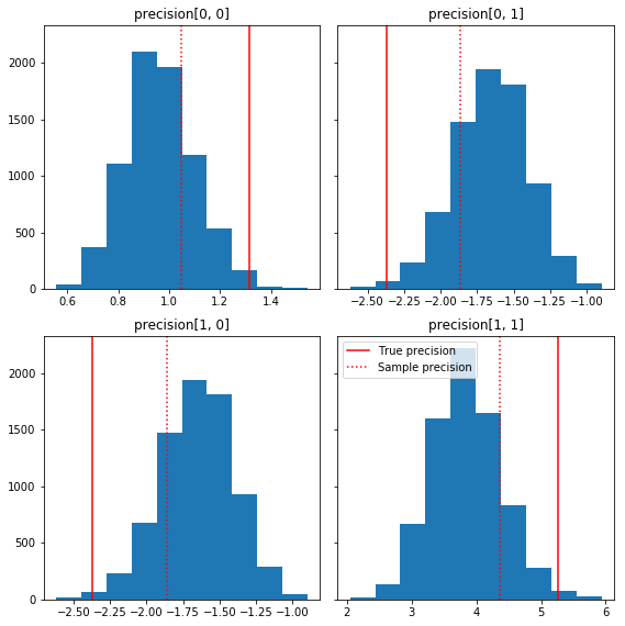
模型批評

如果我們沒有解析解，現在就是進行一些真正的模型批評的時候了。

以下是一些相對於我們的真實值（紅色）的樣本成分的快速直方圖。請注意，樣本已從樣本精度矩陣值向單位矩陣先驗分布收縮。

fig, axes = plt.subplots(2, 2, sharey=True)
fig.set_size_inches(8, 8)
for i in range(2):
  for j in range(2):
    ax = axes[i, j]
    ax.hist(precision_samples_reshaped[:, i, j])
    ax.axvline(true_precision[i, j], color='red',
               label='True precision')
    ax.axvline(sample_precision[i, j], color='red', linestyle=':',
               label='Sample precision')
    ax.set_title('precision[%d, %d]' % (i, j))
plt.tight_layout()
plt.legend()
plt.show()

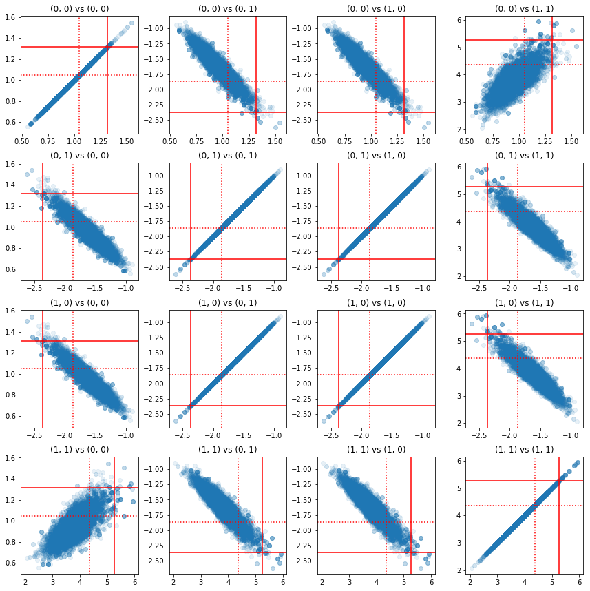
精度成分對的一些散佈圖顯示，由於後驗分布的相關結構，真實後驗分布值並不像上面邊際分布中顯示的那樣不可能。

fig, axes = plt.subplots(4, 4)
fig.set_size_inches(12, 12)
for i1 in range(2):
  for j1 in range(2):
    index1 = 2 * i1 + j1
    for i2 in range(2):
      for j2 in range(2):
        index2 = 2 * i2 + j2
        ax = axes[index1, index2]
        ax.scatter(precision_samples_reshaped[:, i1, j1],
                   precision_samples_reshaped[:, i2, j2], alpha=0.1)
        ax.axvline(true_precision[i1, j1], color='red')
        ax.axhline(true_precision[i2, j2], color='red')
        ax.axvline(sample_precision[i1, j1], color='red', linestyle=':')
        ax.axhline(sample_precision[i2, j2], color='red', linestyle=':')
        ax.set_title('(%d, %d) vs (%d, %d)' % (i1, j1, i2, j2))
plt.tight_layout()
plt.show()

版本 4：更簡單的約束參數抽樣

雙射函數使精度矩陣的抽樣變得簡單明瞭，但是需要相當多的人工轉換到非約束表示形式和從非約束表示形式轉換回來。有一種更簡單的方法！

TransformedTransitionKernel

TransformedTransitionKernel 簡化了此過程。它封裝了您的抽樣器並處理所有轉換。它將雙射函數列表作為引數，這些雙射函數將非約束參數值對應到約束參數值。因此，在這裡我們需要上面使用的 precision_to_unconstrained 雙射函數的反函數。我們可以只使用 tfb.Invert(precision_to_unconstrained)，但這會涉及取反函數的反函數（TensorFlow 不夠聰明，無法將 tf.Invert(tf.Invert()) 簡化為 tf.Identity())，因此我們將改為編寫一個新的雙射函數。

約束雙射函數

# The bijector we need for the TransformedTransitionKernel is the inverse of
# the one we used above
unconstrained_to_precision = tfb.Chain([
    # step 3: take the product of Cholesky factors
    tfb.CholeskyOuterProduct(validate_args=VALIDATE_ARGS),
    # step 2: exponentiate the diagonals    
    tfb.TransformDiagonal(tfb.Exp(validate_args=VALIDATE_ARGS)),
    # step 1: map a vector to a lower triangular matrix
    tfb.FillTriangular(validate_args=VALIDATE_ARGS),
])

# quick sanity check
m = [[1., 2.], [2., 8.]]
m_inv = unconstrained_to_precision.inverse(m).numpy()
m_fwd = unconstrained_to_precision.forward(m_inv).numpy()

print('m:\n', m)
print('unconstrained_to_precision.inverse(m):\n', m_inv)
print('forward(unconstrained_to_precision.inverse(m)):\n', m_fwd)

m:
 [[1.0, 2.0], [2.0, 8.0]]
unconstrained_to_precision.inverse(m):
 [0.6931472 2.        0.       ]
forward(unconstrained_to_precision.inverse(m)):
 [[1. 2.]
 [2. 8.]]

使用 TransformedTransitionKernel 進行抽樣

使用 TransformedTransitionKernel，我們不再需要手動轉換我們的參數。我們的初始值和樣本都是精度矩陣；我們只需要將我們的非約束雙射函數傳遞到核心，它就會處理所有轉換。

@tf.function(autograph=False)
def sample():
  tf.random.set_seed(123)
  log_lik_fn = get_log_lik(my_data)

  # Tuning acceptance rates:
  dtype = np.float32
  num_burnin_iter = 3000
  num_warmup_iter = int(0.8 * num_burnin_iter) 
  num_chain_iter = 2500

  # Set the target average acceptance ratio for the HMC as suggested by
  # Beskos et al. (2013):
  # https://projecteuclid.org/download/pdfview_1/euclid.bj/1383661192
  target_accept_rate = 0.651

  # Initialize the HMC sampler.
  hmc = tfp.mcmc.HamiltonianMonteCarlo(
      target_log_prob_fn=log_lik_fn,
      step_size=0.01,
      num_leapfrog_steps=3)

  ttk = tfp.mcmc.TransformedTransitionKernel(
      inner_kernel=hmc, bijector=unconstrained_to_precision)

  # Adapt the step size using standard adaptive MCMC procedure. See Section 4.2
  # of Andrieu and Thoms (2008):
  # http://www4.ncsu.edu/~rsmith/MA797V_S12/Andrieu08_AdaptiveMCMC_Tutorial.pdf
  adapted_kernel = tfp.mcmc.SimpleStepSizeAdaptation(
      inner_kernel=ttk,
      num_adaptation_steps=num_warmup_iter,
      target_accept_prob=target_accept_rate)

  states = tfp.mcmc.sample_chain(
      num_results=num_chain_iter,
      num_burnin_steps=num_burnin_iter,
      current_state=initial_values,
      kernel=adapted_kernel,
      trace_fn=None,
      parallel_iterations=1)
  # transform samples back to their constrained form
  return states

precision_samples  = sample()

檢查收斂性

\(\hat{R}\) 收斂性檢查看起來不錯！

r_hat = tfp.mcmc.potential_scale_reduction(precision_samples).numpy()
print(r_hat)

[[1.0013582 1.0019467]
 [1.0019467 1.0011805]]

與解析後驗分布比較

再次，讓我們與解析後驗分布進行檢查。

# The output samples have shape [n_steps, n_chains, 2, 2]
# Flatten them to [n_steps * n_chains, 2, 2] via reshape:
precision_samples_reshaped = np.reshape(precision_samples, [-1, 2, 2])

print('True posterior mean:\n', posterior_mean)
print('Mean of samples:\n', np.mean(precision_samples_reshaped, axis=0))

True posterior mean:
 [[ 0.9641779 -1.6534661]
 [-1.6534661  3.8683164]]
Mean of samples:
 [[ 0.96687526 -1.6552585 ]
 [-1.6552585   3.867676  ]]

print('True posterior standard deviation:\n', posterior_sd)
print('Standard deviation of samples:\n', np.std(precision_samples_reshaped, axis=0))

True posterior standard deviation:
 [[0.13435492 0.25050813]
 [0.25050813 0.53903675]]
Standard deviation of samples:
 [[0.13329624 0.24913791]
 [0.24913791 0.53983927]]

最佳化

現在我們已經讓所有東西端對端運行，讓我們做一個更最佳化的版本。對於這個範例來說，速度不太重要，但是一旦矩陣變大，一些最佳化將會產生很大的差異。

我們可以進行的一項重大速度改進是以 Cholesky 分解重新參數化。原因是我們的資料概似函數同時需要共變異數矩陣和精度矩陣。矩陣求逆非常耗時（對於 \(n \times n\) 矩陣為 \(O(n^3)\)），而且如果我們以共變異數矩陣或精度矩陣中的任何一個進行參數化，我們需要執行求逆才能得到另一個。

提醒一下，實數、正定、對稱矩陣 \(M\) 可以分解為 \(M = L L^T\) 形式的乘積，其中矩陣 \(L\) 是下三角矩陣且具有正對角線。給定 \(M\) 的 Cholesky 分解，我們可以更有效率地獲得 \(M\)（下三角矩陣和上三角矩陣的乘積）和 \(M^{-1}\)（透過反向替換）。Cholesky 分解本身的計算成本並不低，但是如果我們以 Cholesky 因子進行參數化，我們只需要計算初始參數值的 Cholesky 分解。

使用共變異數矩陣的 Cholesky 分解

TFP 有一個多元常態分布版本 MultivariateNormalTriL，它是根據共變異數矩陣的 Cholesky 因子進行參數化的。因此，如果我們以共變異數矩陣的 Cholesky 因子進行參數化，我們可以有效率地計算資料對數概似函數。挑戰在於以類似的效率計算先驗對數概似函數。

如果我們有一個適用於樣本 Cholesky 因子的逆 Wishart 分布版本，我們就一切就緒了。唉，我們沒有。（團隊歡迎程式碼提交！）作為替代方案，我們可以結合使用適用於樣本 Cholesky 因子的 Wishart 分布版本和雙射函數鏈。

目前，我們缺少一些標準雙射函數來使事情真正有效率，但是我想展示這個過程作為練習，並說明 TFP 雙射函數的功能。

適用於 Cholesky 因子的 Wishart 分布

Wishart 分布有一個有用的標誌 input_output_cholesky，它指定輸入和輸出矩陣應為 Cholesky 因子。與完整矩陣相比，使用 Cholesky 因子更有效率且在數值上更具優勢，這就是為什麼這是理想的。關於標誌語意的一個重點：它僅表示分布的輸入和輸出的表示形式應更改 - 它不表示分布的完整重新參數化，這將涉及對 log_prob() 函數的 Jacobian 校正。我們實際上想做這個完整的重新參數化，因此我們將建構我們自己的分布。

# An optimized Wishart distribution that has been transformed to operate on
# Cholesky factors instead of full matrices.  Note that we gain a modest
# additional speedup by specifying the Cholesky factor of the scale matrix
# (i.e. by passing in the scale_tril parameter instead of scale).

class CholeskyWishart(tfd.TransformedDistribution):
  """Wishart distribution reparameterized to use Cholesky factors."""
  def __init__(self,
      df,
      scale_tril,
      validate_args=False,
      allow_nan_stats=True,
      name='CholeskyWishart'):
    # Wishart has a bunch of methods that we want to support but not
    # implement.  We'll subclass TransformedDistribution here to take care of
    # those.  We'll override the few for which speed is critical and implement
    # them with a separate Wishart for which input_output_cholesky=True
    super(CholeskyWishart, self).__init__(
        distribution=tfd.WishartTriL(
            df=df,
            scale_tril=scale_tril,
            input_output_cholesky=False,
            validate_args=validate_args,
            allow_nan_stats=allow_nan_stats),
        bijector=tfb.Invert(tfb.CholeskyOuterProduct()),
        validate_args=validate_args,
        name=name
    )
    # Here's the Cholesky distribution we'll use for log_prob() and sample()
    self.cholesky = tfd.WishartTriL(
        df=df,
        scale_tril=scale_tril,
        input_output_cholesky=True,
        validate_args=validate_args,
        allow_nan_stats=allow_nan_stats)

  def _log_prob(self, x):
    return (self.cholesky.log_prob(x) +
            self.bijector.inverse_log_det_jacobian(x, event_ndims=2))

  def _sample_n(self, n, seed=None):
    return self.cholesky._sample_n(n, seed)

# some checks
PRIOR_SCALE_CHOLESKY = np.linalg.cholesky(PRIOR_SCALE)

@tf.function(autograph=False)
def compute_log_prob(m):
  w_transformed = tfd.TransformedDistribution(
      tfd.WishartTriL(df=PRIOR_DF, scale_tril=PRIOR_SCALE_CHOLESKY),
      bijector=tfb.Invert(tfb.CholeskyOuterProduct()))
  w_optimized = CholeskyWishart(
      df=PRIOR_DF, scale_tril=PRIOR_SCALE_CHOLESKY)
  log_prob_transformed = w_transformed.log_prob(m)
  log_prob_optimized = w_optimized.log_prob(m)
  return log_prob_transformed, log_prob_optimized

for matrix in [np.eye(2, dtype=np.float32),
               np.array([[1., 0.], [2., 8.]], dtype=np.float32)]:
  log_prob_transformed, log_prob_optimized = [
      t.numpy() for t in compute_log_prob(matrix)]
  print('Transformed Wishart:', log_prob_transformed)
  print('Optimized Wishart', log_prob_optimized)

Transformed Wishart: -0.84889317
Optimized Wishart -0.84889317
Transformed Wishart: -99.269455
Optimized Wishart -99.269455

建構逆 Wishart 分布

我們將共變異數矩陣 \(C\) 分解為 \(C = L L^T\)，其中 \(L\) 是下三角矩陣且具有正對角線。我們想知道 \(L\) 的機率，假設 \(C \sim W^{-1}(\nu, V)\)，其中 \(W^{-1}\) 是逆 Wishart 分布。

逆 Wishart 分布具有以下屬性：如果 \(C \sim W^{-1}(\nu, V)\)，則精度矩陣 \(C^{-1} \sim W(\nu, V^{-1})\)。因此，我們可以透過 TransformedDistribution 獲得 \(L\) 的機率，它將 Wishart 分布和雙射函數作為參數，該雙射函數將精度矩陣的 Cholesky 因子對應到其反函數的 Cholesky 因子。

從 \(C^{-1}\) 的 Cholesky 因子獲得 \(L\) 的一種直接（但效率不高）的方法是透過反向求解來反轉 Cholesky 因子，然後從這些反轉的因子形成共變異數矩陣，然後執行 Cholesky 分解。

讓 \(C^{-1} = M M^T\) 的 Cholesky 分解。\(M\) 是下三角矩陣，因此我們可以使用 MatrixInverseTriL 雙射函數來反轉它。

從 \(M^{-1}\) 形成 \(C\) 有點棘手：\(C = (M M^T)^{-1} = M^{-T}M^{-1} = M^{-T} (M^{-T})^T\)。\(M\) 是下三角矩陣，因此 \(M^{-1}\) 也將是下三角矩陣，而 \(M^{-T}\) 將是上三角矩陣。CholeskyOuterProduct() 雙射函數僅適用於下三角矩陣，因此我們無法使用它從 \(M^{-T}\) 形成 \(C\)。我們的變通方法是一系列雙射函數，它們排列矩陣的行和列。

幸運的是，此邏輯封裝在 CholeskyToInvCholesky 雙射函數中！

組合所有部分

# verify that the bijector works
m = np.array([[1., 0.], [2., 8.]], dtype=np.float32)
c_inv = m.dot(m.T)
c = np.linalg.inv(c_inv)
c_chol = np.linalg.cholesky(c)
wishart_cholesky_to_iw_cholesky = tfb.CholeskyToInvCholesky()
w_fwd = wishart_cholesky_to_iw_cholesky.forward(m).numpy()

print('numpy =\n', c_chol)
print('bijector =\n', w_fwd)

numpy =
 [[ 1.0307764   0.        ]
 [-0.03031695  0.12126781]]
bijector =
 [[ 1.0307764   0.        ]
 [-0.03031695  0.12126781]]

我們的最終分布

我們在 Cholesky 因子上運算的逆 Wishart 分布如下：

inverse_wishart_cholesky = tfd.TransformedDistribution(
    distribution=CholeskyWishart(
        df=PRIOR_DF,
        scale_tril=np.linalg.cholesky(np.linalg.inv(PRIOR_SCALE))),
    bijector=tfb.CholeskyToInvCholesky())

我們得到了逆 Wishart 分布，但是它有點慢，因為我們必須在雙射函數中執行 Cholesky 分解。讓我們回到精度矩陣參數化，看看我們可以在那裡做些什麼來進行最佳化。

最終（！）版本：使用精度矩陣的 Cholesky 分解

另一種方法是使用精度矩陣的 Cholesky 因子。在這裡，先驗概似函數很容易計算，但是資料對數概似函數需要更多工作，因為 TFP 沒有由精度參數化的多元常態分布版本。

最佳化先驗對數概似函數

我們使用上面建構的 CholeskyWishart 分布來建構先驗分布。

# Our new prior.
PRIOR_SCALE_CHOLESKY = np.linalg.cholesky(PRIOR_SCALE)

def log_lik_prior_cholesky(precisions_cholesky):
  rv_precision = CholeskyWishart(
      df=PRIOR_DF,
      scale_tril=PRIOR_SCALE_CHOLESKY,
      validate_args=VALIDATE_ARGS,
      allow_nan_stats=ALLOW_NAN_STATS)
  return rv_precision.log_prob(precisions_cholesky)

# Check against the slower TF implementation and the NumPy implementation.
# Note that when comparing to NumPy, we need to add in the Jacobian correction.
precisions = [np.eye(2, dtype=np.float32),
              true_precision]
precisions_cholesky = np.stack([np.linalg.cholesky(m) for m in precisions])
precisions = np.stack(precisions)
lik_tf = log_lik_prior_cholesky(precisions_cholesky).numpy()
lik_tf_slow = tfd.TransformedDistribution(
    distribution=tfd.WishartTriL(
        df=PRIOR_DF, scale_tril=tf.linalg.cholesky(PRIOR_SCALE)),
    bijector=tfb.Invert(tfb.CholeskyOuterProduct())).log_prob(
    precisions_cholesky).numpy()
corrections = tfb.Invert(tfb.CholeskyOuterProduct()).inverse_log_det_jacobian(
    precisions_cholesky, event_ndims=2).numpy()
n = precisions.shape[0]

for i in range(n):
  print(i)
  print('numpy:', log_lik_prior_numpy(precisions[i]) + corrections[i])
  print('tensorflow slow:', lik_tf_slow[i])
  print('tensorflow fast:', lik_tf[i])

0
numpy: -0.8488930160357633
tensorflow slow: -0.84889317
tensorflow fast: -0.84889317
1
numpy: -7.442875031036973
tensorflow slow: -7.442877
tensorflow fast: -7.442876

最佳化資料對數概似函數

我們可以使用 TFP 的雙射函數來建構我們自己的多元常態分布版本。以下是關鍵想法：

假設我有一個列向量 \(X\)，其元素是 \(N(0, 1)\) 的 iid 樣本。我們有 \(\text{mean}(X) = 0\) 和 \(\text{cov}(X) = I\)

現在讓 \(Y = A X + b\)。我們有 \(\text{mean}(Y) = b\) 和 \(\text{cov}(Y) = A A^T\)

因此，我們可以透過對 iid 標準常態樣本向量使用仿射變換 \(Ax+b\)，來產生具有平均值 \(b\) 和共變異數 \(C\) 的向量，前提是 \(A A^T = C\)。\(C\) 的 Cholesky 分解具有所需的屬性。但是，還有其他解決方案。

讓 \(P = C^{-1}\)，並讓 \(P\) 的 Cholesky 分解為 \(B\)，即 \(B B^T = P\)。現在

\(P^{-1} = (B B^T)^{-1} = B^{-T} B^{-1} = B^{-T} (B^{-T})^T\)

因此，獲得我們期望的平均值和共變異數的另一種方法是使用仿射變換 \(Y=B^{-T}X + b\)。

我們的方法（由 此筆記本 提供）：

1. 使用 tfd.Independent() 將一批 1-D Normal 隨機變數組合為單個多維隨機變數。Independent() 的 reinterpreted_batch_ndims 參數指定應重新解釋為事件維度的批次維度數。在我們的例子中，我們建立一個長度為 2 的 1-D 批次，我們將其轉換為長度為 2 的 1-D 事件，因此 reinterpreted_batch_ndims=1。
2. 應用雙射函數以新增所需的共變異數：tfb.Invert(tfb.ScaleMatvecTriL(scale_tril=precision_cholesky, adjoint=True))。請注意，在上面，我們將 iid 常態隨機變數乘以精度矩陣 Cholesky 因子的反函數的轉置 \((B^{-T}X)\)。tfb.Invert 負責反轉 \(B\)，而 adjoint=True 標誌執行轉置。
3. 應用雙射函數以新增所需的偏移量：tfb.Shift(shift=shift) 請注意，我們必須將偏移量作為與初始反轉仿射變換分開的步驟來執行，否則反轉比例會應用於偏移量（因為 \(y=Ax+b\) 的反函數是 \(x=A^{-1}y - A^{-1}b\））。

class MVNPrecisionCholesky(tfd.TransformedDistribution):
  """Multivariate normal parameterized by loc and Cholesky precision matrix."""

  def __init__(self, loc, precision_cholesky, name=None):
    super(MVNPrecisionCholesky, self).__init__(
        distribution=tfd.Independent(
            tfd.Normal(loc=tf.zeros_like(loc),
                       scale=tf.ones_like(loc)),
            reinterpreted_batch_ndims=1),
        bijector=tfb.Chain([
            tfb.Shift(shift=loc),
            tfb.Invert(tfb.ScaleMatvecTriL(scale_tril=precision_cholesky,
                                  adjoint=True)),
        ]),
        name=name)

@tf.function(autograph=False)
def log_lik_data_cholesky(precisions_cholesky, replicated_data):
  n = tf.shape(precisions_cholesky)[0]  # number of precision matrices
  rv_data = MVNPrecisionCholesky(
      loc=tf.zeros([n, 2]),
      precision_cholesky=precisions_cholesky)
  return tf.reduce_sum(rv_data.log_prob(replicated_data), axis=0)

# check against the numpy implementation
true_precision_cholesky = np.linalg.cholesky(true_precision)
precisions = [np.eye(2, dtype=np.float32), true_precision]
precisions_cholesky = np.stack([np.linalg.cholesky(m) for m in precisions])
precisions = np.stack(precisions)
n = precisions_cholesky.shape[0]
replicated_data = np.tile(np.expand_dims(my_data, axis=1), reps=[1, 2, 1])
lik_tf = log_lik_data_cholesky(precisions_cholesky, replicated_data).numpy()

for i in range(n):
  print(i)
  print('numpy:', log_lik_data_numpy(precisions[i], my_data))
  print('tensorflow:', lik_tf[i])

0
numpy: -430.71218815801365
tensorflow: -430.71207
1
numpy: -280.81822950593767
tensorflow: -280.81824

組合對數概似函數

現在我們將先驗對數概似函數和資料對數概似函數組合在閉包中。

def get_log_lik_cholesky(data, n_chains=1):
  # The data argument that is passed in will be available to the inner function
  # below so it doesn't have to be passed in as a parameter.
  replicated_data = np.tile(np.expand_dims(data, axis=1), reps=[1, n_chains, 1])

  @tf.function(autograph=False)
  def _log_lik_cholesky(precisions_cholesky):
    return (log_lik_data_cholesky(precisions_cholesky, replicated_data) +
            log_lik_prior_cholesky(precisions_cholesky))

  return _log_lik_cholesky

約束雙射函數

我們的樣本被約束為有效的 Cholesky 因子，這表示它們必須是具有正對角線的下三角矩陣。TransformedTransitionKernel 需要一個雙射函數，該函數將非約束張量對應到具有我們所需約束的張量和從具有我們所需約束的張量對應到非約束張量。我們已從雙射函數的反函數中移除 Cholesky 分解，這加快了速度。

unconstrained_to_precision_cholesky = tfb.Chain([
    # step 2: exponentiate the diagonals    
    tfb.TransformDiagonal(tfb.Exp(validate_args=VALIDATE_ARGS)),
    # step 1: expand the vector to a lower triangular matrix
    tfb.FillTriangular(validate_args=VALIDATE_ARGS),
])

# some checks
inv = unconstrained_to_precision_cholesky.inverse(precisions_cholesky).numpy()
fwd = unconstrained_to_precision_cholesky.forward(inv).numpy()
print('precisions_cholesky:\n', precisions_cholesky)
print('\ninv:\n', inv)
print('\nfwd(inv):\n', fwd)

precisions_cholesky:
 [[[ 1.         0.       ]
  [ 0.         1.       ]]

 [[ 1.1470785  0.       ]
  [-2.0647411  1.0000004]]]

inv:
 [[ 0.0000000e+00  0.0000000e+00  0.0000000e+00]
 [ 3.5762781e-07 -2.0647411e+00  1.3721828e-01]]

fwd(inv):
 [[[ 1.         0.       ]
  [ 0.         1.       ]]

 [[ 1.1470785  0.       ]
  [-2.0647411  1.0000004]]]

初始值

我們產生一個初始值張量。我們正在使用 Cholesky 因子，因此我們產生一些 Cholesky 因子初始值。

# The number of chains is determined by the shape of the initial values.
# Here we'll generate 3 chains, so we'll need a tensor of 3 initial values.
N_CHAINS = 3

np.random.seed(123)

initial_values_cholesky = []
for i in range(N_CHAINS):
  initial_values_cholesky.append(np.array(
      [[0.5 + np.random.uniform(), 0.0],
       [-0.5 + np.random.uniform(), 0.5 + np.random.uniform()]],
      dtype=np.float32))
initial_values_cholesky = np.stack(initial_values_cholesky)

抽樣

我們使用 TransformedTransitionKernel 抽樣 N_CHAINS 鏈。

@tf.function(autograph=False)
def sample():
  tf.random.set_seed(123)
  log_lik_fn = get_log_lik_cholesky(my_data)

  # Tuning acceptance rates:
  dtype = np.float32
  num_burnin_iter = 3000
  num_warmup_iter = int(0.8 * num_burnin_iter) 
  num_chain_iter = 2500

  # Set the target average acceptance ratio for the HMC as suggested by
  # Beskos et al. (2013):
  # https://projecteuclid.org/download/pdfview_1/euclid.bj/1383661192
  target_accept_rate = 0.651

  # Initialize the HMC sampler.
  hmc = tfp.mcmc.HamiltonianMonteCarlo(
      target_log_prob_fn=log_lik_fn,
      step_size=0.01,
      num_leapfrog_steps=3)

  ttk = tfp.mcmc.TransformedTransitionKernel(
      inner_kernel=hmc, bijector=unconstrained_to_precision_cholesky)

  # Adapt the step size using standard adaptive MCMC procedure. See Section 4.2
  # of Andrieu and Thoms (2008):
  # http://www4.ncsu.edu/~rsmith/MA797V_S12/Andrieu08_AdaptiveMCMC_Tutorial.pdf
  adapted_kernel = tfp.mcmc.SimpleStepSizeAdaptation(
      inner_kernel=ttk,
      num_adaptation_steps=num_warmup_iter,
      target_accept_prob=target_accept_rate)

  states = tfp.mcmc.sample_chain(
      num_results=num_chain_iter,
      num_burnin_steps=num_burnin_iter,
      current_state=initial_values,
      kernel=adapted_kernel,
      trace_fn=None,
      parallel_iterations=1)
  # transform samples back to their constrained form
  samples = tf.linalg.matmul(states, states, transpose_b=True)
  return samples

precision_samples = sample()

收斂性檢查

快速收斂性檢查看起來不錯

r_hat = tfp.mcmc.potential_scale_reduction(precision_samples).numpy()
print(r_hat)

[[1.0013583 1.0019467]
 [1.0019467 1.0011804]]

將結果與解析後驗分布進行比較

# The output samples have shape [n_steps, n_chains, 2, 2]
# Flatten them to [n_steps * n_chains, 2, 2] via reshape:
precision_samples_reshaped = np.reshape(precision_samples, newshape=[-1, 2, 2])

再次，樣本平均值和標準差與解析後驗分布的平均值和標準差相符。

print('True posterior mean:\n', posterior_mean)
print('Mean of samples:\n', np.mean(precision_samples_reshaped, axis=0))

True posterior mean:
 [[ 0.9641779 -1.6534661]
 [-1.6534661  3.8683164]]
Mean of samples:
 [[ 0.9668749 -1.6552604]
 [-1.6552604  3.8676758]]

print('True posterior standard deviation:\n', posterior_sd)
print('Standard deviation of samples:\n', np.std(precision_samples_reshaped, axis=0))

True posterior standard deviation:
 [[0.13435492 0.25050813]
 [0.25050813 0.53903675]]
Standard deviation of samples:
 [[0.13329637 0.24913797]
 [0.24913797 0.53983945]]

好的，全部完成！我們已讓最佳化抽樣器正常運作。