TFP 版本說明筆記本 (0.13.0)

此筆記本的目的是透過一些小程式碼片段來協助 TFP 0.13.0「活起來」- 示範您可以使用 TFP 達成的目標。

在 TensorFlow.org 上檢視

在 Google Colab 中執行

在 GitHub 上檢視原始碼

下載筆記本

安裝與匯入

!pip3 install -qU tensorflow==2.5.0 tensorflow_probability==0.13.0 tensorflow-datasets inference_gym

import tensorflow as tf
import tensorflow_probability as tfp
assert '0.13' in tfp.__version__, tfp.__version__
assert '2.5' in tf.__version__, tf.__version__

physical_devices = tf.config.list_physical_devices('CPU')
tf.config.set_logical_device_configuration(
    physical_devices[0],
    [tf.config.LogicalDeviceConfiguration(),
     tf.config.LogicalDeviceConfiguration()])

tfd = tfp.distributions
tfb = tfp.bijectors
tfpk = tfp.math.psd_kernels

import matplotlib.pyplot as plt
import numpy as np
import scipy.interpolate
import IPython
import seaborn as sns
import logging

|████████████████████████████████| 5.4MB 8.8MB/s 
     |████████████████████████████████| 3.9MB 37.1MB/s 
     |████████████████████████████████| 296kB 31.6MB/s

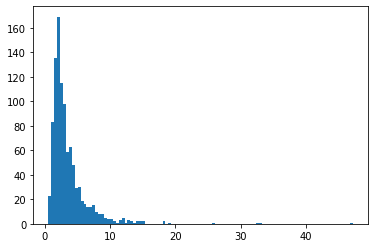
分佈 [核心數學]

`BetaQuotient`

兩個獨立 Beta 分佈隨機變數的比率

plt.hist(tfd.BetaQuotient(concentration1_numerator=5.,
                          concentration0_numerator=2.,
                          concentration1_denominator=3.,
                          concentration0_denominator=8.).sample(1_000, seed=(1, 23)),
         bins='auto');

png

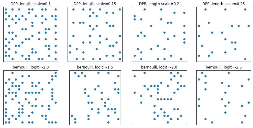
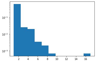
`DeterminantalPointProcess`

給定集合的子集（表示為 one-hot）分佈。樣本遵循排斥性屬性 (機率與所選點子集對應向量跨越的體積成正比)，這趨向於採樣多樣化的子集。[與獨立且相同分佈的白努利樣本比較。]

grid_size = 16
# Generate grid_size**2 pts on the unit square.
grid = np.arange(0, 1, 1./grid_size).astype(np.float32)
import itertools
points = np.array(list(itertools.product(grid, grid)))

# Create the kernel L that parameterizes the DPP.
kernel_amplitude = 2.
kernel_lengthscale = [.1, .15, .2, .25]  # Increasing length scale indicates more points are "nearby", tending toward smaller subsets.
kernel = tfpk.ExponentiatedQuadratic(kernel_amplitude, kernel_lengthscale)
kernel_matrix = kernel.matrix(points, points)

eigenvalues, eigenvectors = tf.linalg.eigh(kernel_matrix)
dpp = tfd.DeterminantalPointProcess(eigenvalues, eigenvectors)
print(dpp)

# The inner-most dimension of the result of `dpp.sample` is a multi-hot
# encoding of a subset of {1, ..., ground_set_size}.
# We will compare against a bernoulli distribution.
samps_dpp = dpp.sample(seed=(1, 2))  # 4 x grid_size**2
logits = tf.broadcast_to([[-1.], [-1.5], [-2], [-2.5]], [4, grid_size**2])
samps_bern = tfd.Bernoulli(logits=logits).sample(seed=(2, 3))

plt.figure(figsize=(12, 6))
for i, (samp, samp_bern) in enumerate(zip(samps_dpp, samps_bern)):
  plt.subplot(241 + i)
  plt.scatter(*points[np.where(samp)].T)
  plt.title(f'DPP, length scale={kernel_lengthscale[i]}')
  plt.xticks([])
  plt.yticks([])
  plt.gca().set_aspect(1.)
  plt.subplot(241 + i + 4)
  plt.scatter(*points[np.where(samp_bern)].T)
  plt.title(f'bernoulli, logit={logits[i,0]}')
  plt.xticks([])
  plt.yticks([])
  plt.gca().set_aspect(1.)

plt.tight_layout()
plt.show()

tfp.distributions.DeterminantalPointProcess("DeterminantalPointProcess", batch_shape=[4], event_shape=[256], dtype=int32)

png

`SigmoidBeta`

兩個 Gamma 分佈的對數勝算比。比 Beta 具有更數值穩定的樣本空間。

plt.hist(tfd.SigmoidBeta(concentration1=.01, concentration0=2.).sample(10_000, seed=(1, 23)),
         bins='auto', density=True);
plt.show()

print('Old way, fractions non-finite:')
print(np.sum(~tf.math.is_finite(
    tfb.Invert(tfb.Sigmoid())(tfd.Beta(concentration1=.01, concentration0=2.)).sample(10_000, seed=(1, 23)))) / 10_000)
print(np.sum(~tf.math.is_finite(
    tfb.Invert(tfb.Sigmoid())(tfd.Beta(concentration1=2., concentration0=.01)).sample(10_000, seed=(2, 34)))) / 10_000)

png

Old way, fractions non-finite:
0.4215
0.8624

Zipf

新增 JAX 支援。

plt.hist(tfd.Zipf(3.).sample(1_000, seed=(12, 34)).numpy(), bins='auto', density=True, log=True);

png

`NormalInverseGaussian`

支援肥尾、偏斜和標準常態分佈的彈性參數族。

`MatrixNormalLinearOperator`

矩陣常態分佈。

# Initialize a single 2 x 3 Matrix Normal.
mu = [[1., 2, 3], [3., 4, 5]]
col_cov = [[ 0.36,  0.12,  0.06],
           [ 0.12,  0.29, -0.13],
           [ 0.06, -0.13,  0.26]]
scale_column = tf.linalg.LinearOperatorLowerTriangular(tf.linalg.cholesky(col_cov))
scale_row = tf.linalg.LinearOperatorDiag([0.9, 0.8])

mvn = tfd.MatrixNormalLinearOperator(loc=mu, scale_row=scale_row, scale_column=scale_column)
mvn.sample()

WARNING:tensorflow:From /usr/local/lib/python3.7/dist-packages/tensorflow/python/ops/linalg/linear_operator_kronecker.py:224: LinearOperator.graph_parents (from tensorflow.python.ops.linalg.linear_operator) is deprecated and will be removed in a future version.
Instructions for updating:
Do not call `graph_parents`.
<tf.Tensor: shape=(2, 3), dtype=float32, numpy=
array([[1.2495145, 1.549366 , 3.2748342],
       [3.7330258, 4.3413105, 4.83423  ]], dtype=float32)>

`MatrixStudentTLinearOperator`

矩陣 T 分佈。

mu = [[1., 2, 3], [3., 4, 5]]
col_cov = [[ 0.36,  0.12,  0.06],
           [ 0.12,  0.29, -0.13],
           [ 0.06, -0.13,  0.26]]
scale_column = tf.linalg.LinearOperatorLowerTriangular(tf.linalg.cholesky(col_cov))
scale_row = tf.linalg.LinearOperatorDiag([0.9, 0.8])

mvn = tfd.MatrixTLinearOperator(
    df=2.,
    loc=mu,
    scale_row=scale_row,
    scale_column=scale_column)
mvn.sample()

<tf.Tensor: shape=(2, 3), dtype=float32, numpy=
array([[1.6549466, 2.6708362, 2.8629923],
       [2.1222284, 3.6904747, 5.08014  ]], dtype=float32)>

分佈 [軟體/包裝函式]

`Sharded`

跨多個處理器分片分佈的獨立事件部分。彙總跨裝置的 log_prob，與 tfp.experimental.distribute.JointDistribution* 協調處理梯度。在「分散式推論」筆記本中有更多資訊。

strategy = tf.distribute.MirroredStrategy()

@tf.function
def sample_and_lp(seed):
  d = tfp.experimental.distribute.Sharded(tfd.Normal(0, 1))
  s = d.sample(seed=seed)
  return s, d.log_prob(s)

strategy.run(sample_and_lp, args=(tf.constant([12,34]),))

WARNING:tensorflow:There are non-GPU devices in `tf.distribute.Strategy`, not using nccl allreduce.
WARNING:tensorflow:Collective ops is not configured at program startup. Some performance features may not be enabled.
INFO:tensorflow:Using MirroredStrategy with devices ('/job:localhost/replica:0/task:0/device:CPU:0', '/job:localhost/replica:0/task:0/device:CPU:1')
INFO:tensorflow:Reduce to /job:localhost/replica:0/task:0/device:CPU:0 then broadcast to ('/job:localhost/replica:0/task:0/device:CPU:0', '/job:localhost/replica:0/task:0/device:CPU:1').
(PerReplica:{
   0: <tf.Tensor: shape=(), dtype=float32, numpy=0.0051413667>,
   1: <tf.Tensor: shape=(), dtype=float32, numpy=-0.3393052>
 }, PerReplica:{
   0: <tf.Tensor: shape=(), dtype=float32, numpy=-1.8954543>,
   1: <tf.Tensor: shape=(), dtype=float32, numpy=-1.8954543>
 })

`BatchBroadcast`

隱含廣播基礎分佈的批次維度與給定的批次形狀或到給定的批次形狀。

underlying = tfd.MultivariateNormalDiag(tf.zeros([7, 1, 5]), tf.ones([5]))
print('underlying:', underlying)

d = tfd.BatchBroadcast(underlying, [8, 1, 6])
print('broadcast [7, 1] *with* [8, 1, 6]:', d)

try:
  tfd.BatchBroadcast(underlying, to_shape=[8, 1, 6])
except ValueError as e:
  print('broadcast [7, 1] *to* [8, 1, 6] is invalid:', e)

d = tfd.BatchBroadcast(underlying, to_shape=[8, 7, 6])
print('broadcast [7, 1] *to* [8, 7, 6]:', d)

underlying: tfp.distributions.MultivariateNormalDiag("MultivariateNormalDiag", batch_shape=[7, 1], event_shape=[5], dtype=float32)
broadcast [7, 1] *with* [8, 1, 6]: tfp.distributions.BatchBroadcast("BatchBroadcastMultivariateNormalDiag", batch_shape=[8, 7, 6], event_shape=[5], dtype=float32)
broadcast [7, 1] *to* [8, 1, 6] is invalid: Argument `to_shape` ([8 1 6]) is incompatible with underlying distribution batch shape ((7, 1)).
broadcast [7, 1] *to* [8, 7, 6]: tfp.distributions.BatchBroadcast("BatchBroadcastMultivariateNormalDiag", batch_shape=[8, 7, 6], event_shape=[5], dtype=float32)

`Masked`

對於單一程式/多重資料或稀疏即遮罩密集使用案例，遮罩無效基礎分佈 log_prob 的分佈。

d = tfd.Masked(tfd.Normal(tf.zeros([7]), 1), 
               validity_mask=tf.sequence_mask([3, 4], 7))
print(d.log_prob(d.sample(seed=(1, 1))))

d = tfd.Masked(tfd.Normal(0, 1), 
               validity_mask=[False, True, False],
               safe_sample_fn=tfd.Distribution.mode)
print(d.log_prob(d.sample(seed=(2, 2))))

tf.Tensor(
[[-2.3054113 -1.8524303 -1.2220721  0.         0.         0.

   0.       ]
 [-1.118623  -1.1370811 -1.1574132 -5.884986   0.         0.
   0.       ]], shape=(2, 7), dtype=float32)
tf.Tensor([ 0.         -0.93683904  0.        ], shape=(3,), dtype=float32)

雙射器

雙射器
- 新增雙射器以模仿 tf.nest.flatten (tfb.tree_flatten) 和 tf.nest.pack_sequence_as (tfb.pack_sequence_as)。
- 新增 tfp.experimental.bijectors.Sharded
- 移除已淘汰的 tfb.ScaleTrilL。改用 tfb.FillScaleTriL。
- 為雙射器新增 cls.parameter_properties() 註解。
- 將範圍 tfb.Power 擴充到所有奇數整數冪的實數。
- 如果未另行指定，則使用自動微分推斷純量雙射器的對數行列式 Jacobian。

重組雙射器

ex = (tf.constant(1.), dict(b=tf.constant(2.), c=tf.constant(3.)))
b = tfb.tree_flatten(ex)
print(b.forward(ex))
print(b.inverse(list(tf.constant([1., 2, 3]))))

b = tfb.pack_sequence_as(ex)
print(b.forward(list(tf.constant([1., 2, 3]))))
print(b.inverse(ex))

[<tf.Tensor: shape=(), dtype=float32, numpy=1.0>, <tf.Tensor: shape=(), dtype=float32, numpy=2.0>, <tf.Tensor: shape=(), dtype=float32, numpy=3.0>]
(<tf.Tensor: shape=(), dtype=float32, numpy=1.0>, {'b': <tf.Tensor: shape=(), dtype=float32, numpy=2.0>, 'c': <tf.Tensor: shape=(), dtype=float32, numpy=3.0>})
(<tf.Tensor: shape=(), dtype=float32, numpy=1.0>, {'b': <tf.Tensor: shape=(), dtype=float32, numpy=2.0>, 'c': <tf.Tensor: shape=(), dtype=float32, numpy=3.0>})
[<tf.Tensor: shape=(), dtype=float32, numpy=1.0>, <tf.Tensor: shape=(), dtype=float32, numpy=2.0>, <tf.Tensor: shape=(), dtype=float32, numpy=3.0>]

`Sharded`

對數行列式中的 SPMD 縮減。請參閱下方的「分佈」中的 Sharded。

strategy = tf.distribute.MirroredStrategy()

def sample_lp_logdet(seed):
  d = tfd.TransformedDistribution(tfp.experimental.distribute.Sharded(tfd.Normal(0, 1), shard_axis_name='i'),
                                  tfp.experimental.bijectors.Sharded(tfb.Sigmoid(), shard_axis_name='i'))
  s = d.sample(seed=seed)
  return s, d.log_prob(s), d.bijector.inverse_log_det_jacobian(s)
strategy.run(sample_lp_logdet, (tf.constant([1, 2]),))

WARNING:tensorflow:There are non-GPU devices in `tf.distribute.Strategy`, not using nccl allreduce.
WARNING:tensorflow:Collective ops is not configured at program startup. Some performance features may not be enabled.
INFO:tensorflow:Using MirroredStrategy with devices ('/job:localhost/replica:0/task:0/device:CPU:0', '/job:localhost/replica:0/task:0/device:CPU:1')
WARNING:tensorflow:Using MirroredStrategy eagerly has significant overhead currently. We will be working on improving this in the future, but for now please wrap `call_for_each_replica` or `experimental_run` or `run` inside a tf.function to get the best performance.
INFO:tensorflow:Reduce to /job:localhost/replica:0/task:0/device:CPU:0 then broadcast to ('/job:localhost/replica:0/task:0/device:CPU:0', '/job:localhost/replica:0/task:0/device:CPU:1').
INFO:tensorflow:Reduce to /job:localhost/replica:0/task:0/device:CPU:0 then broadcast to ('/job:localhost/replica:0/task:0/device:CPU:0', '/job:localhost/replica:0/task:0/device:CPU:1').
(PerReplica:{
   0: <tf.Tensor: shape=(), dtype=float32, numpy=0.87746525>,
   1: <tf.Tensor: shape=(), dtype=float32, numpy=0.24580425>
 }, PerReplica:{
   0: <tf.Tensor: shape=(), dtype=float32, numpy=-0.48870325>,
   1: <tf.Tensor: shape=(), dtype=float32, numpy=-0.48870325>
 }, PerReplica:{
   0: <tf.Tensor: shape=(), dtype=float32, numpy=3.9154015>,
   1: <tf.Tensor: shape=(), dtype=float32, numpy=3.9154015>
 })

VI

將 build_split_flow_surrogate_posterior 新增至 tfp.experimental.vi，以從正規化流建構結構化 VI 替代後驗。
將 build_affine_surrogate_posterior 新增至 tfp.experimental.vi，以從事件形狀建構 ADVI 替代後驗。
將 build_affine_surrogate_posterior_from_base_distribution 新增至 tfp.experimental.vi，以使用仿射轉換引發的相關結構啟用 ADVI 替代後驗的建構。

VI/MAP/MLE

新增便利方法 tfp.experimental.util.make_trainable(cls)，以建立分佈和雙射器的可訓練執行個體。

d = tfp.experimental.util.make_trainable(tfd.Gamma)
print(d.trainable_variables)
print(d)

(<tf.Variable 'Gamma_trainable_variables/concentration:0' shape=() dtype=float32, numpy=1.0296053>, <tf.Variable 'Gamma_trainable_variables/log_rate:0' shape=() dtype=float32, numpy=-0.3465951>)
tfp.distributions.Gamma("Gamma", batch_shape=[], event_shape=[], dtype=float32)

MCMC

MCMC 診斷支援任意狀態結構，而不僅僅是清單。
remc_thermodynamic_integrals 已新增至 tfp.experimental.mcmc
新增 tfp.experimental.mcmc.windowed_adaptive_hmc
新增實驗性 API，用於從不受限制空間中接近零的均勻分佈初始化馬可夫鏈。tfp.experimental.mcmc.init_near_unconstrained_zero
新增實驗性公用程式，用於重試馬可夫鏈初始化，直到找到可接受的點。tfp.experimental.mcmc.retry_init
改組實驗性串流 MCMC API，以最少的干擾插入 tfp.mcmc。
將 ThinningKernel 新增至 experimental.mcmc。
新增 experimental.mcmc.run_kernel 驅動程式，作為 mcmc.sample_chain 的候選串流式取代項目

`init_near_unconstrained_zero`、`retry_init`

@tfd.JointDistributionCoroutine
def model():
  Root = tfd.JointDistributionCoroutine.Root
  c0 = yield Root(tfd.Gamma(2, 2, name='c0'))
  c1 = yield Root(tfd.Gamma(2, 2, name='c1'))
  counts = yield tfd.Sample(tfd.BetaBinomial(23, c1, c0), 10, name='counts')
jd = model.experimental_pin(counts=model.sample(seed=[20, 30]).counts)

init_dist = tfp.experimental.mcmc.init_near_unconstrained_zero(jd)
print(init_dist)

tfp.experimental.mcmc.retry_init(init_dist.sample, jd.unnormalized_log_prob)

tfp.distributions.TransformedDistribution("default_joint_bijectorrestructureJointDistributionSequential", batch_shape=StructTuple(
  c0=[],
  c1=[]
), event_shape=StructTuple(
  c0=[],
  c1=[]
), dtype=StructTuple(
  c0=float32,
  c1=float32
))
StructTuple(
  c0=<tf.Tensor: shape=(), dtype=float32, numpy=1.7879653>,
  c1=<tf.Tensor: shape=(), dtype=float32, numpy=0.34548905>
)

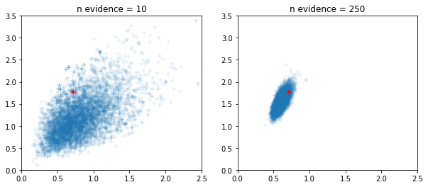
視窗化自適應 HMC 和 NUTS 採樣器

fig, ax = plt.subplots(1, 2, figsize=(10, 4))
for i, n_evidence in enumerate((10, 250)):
  ax[i].set_title(f'n evidence = {n_evidence}')
  ax[i].set_xlim(0, 2.5); ax[i].set_ylim(0, 3.5)
  @tfd.JointDistributionCoroutine
  def model():
    Root = tfd.JointDistributionCoroutine.Root
    c0 = yield Root(tfd.Gamma(2, 2, name='c0'))
    c1 = yield Root(tfd.Gamma(2, 2, name='c1'))
    counts = yield tfd.Sample(tfd.BetaBinomial(23, c1, c0), n_evidence, name='counts')
  s = model.sample(seed=[20, 30])
  print(s)
  jd = model.experimental_pin(counts=s.counts)
  states, trace = tf.function(tfp.experimental.mcmc.windowed_adaptive_hmc)(
      100, jd, num_leapfrog_steps=5, seed=[100, 200])
  ax[i].scatter(states.c0.numpy().reshape(-1), states.c1.numpy().reshape(-1), 
                marker='+', alpha=.1)
  ax[i].scatter(s.c0, s.c1, marker='+', color='r')

StructTuple(
  c0=<tf.Tensor: shape=(), dtype=float32, numpy=0.7161876>,
  c1=<tf.Tensor: shape=(), dtype=float32, numpy=1.7696666>,
  counts=<tf.Tensor: shape=(10,), dtype=float32, numpy=array([ 6., 10., 23.,  7.,  2., 20., 14., 16., 22., 17.], dtype=float32)>
)
WARNING:tensorflow:6 out of the last 6 calls to <function windowed_adaptive_hmc at 0x7fda42bed8c0> triggered tf.function retracing. Tracing is expensive and the excessive number of tracings could be due to (1) creating @tf.function repeatedly in a loop, (2) passing tensors with different shapes, (3) passing Python objects instead of tensors. For (1), please define your @tf.function outside of the loop. For (2), @tf.function has reduce_retracing=True option that relaxes argument shapes that can avoid unnecessary retracing. For (3), please refer to https://tensorflow.dev.org.tw/guide/function#controlling_retracing and https://tensorflow.dev.org.tw/api_docs/python/tf/function for  more details.
StructTuple(
  c0=<tf.Tensor: shape=(), dtype=float32, numpy=0.7161876>,
  c1=<tf.Tensor: shape=(), dtype=float32, numpy=1.7696666>,
  counts=<tf.Tensor: shape=(250,), dtype=float32, numpy=
    array([ 6., 10., 23.,  7.,  2., 20., 14., 16., 22., 17., 22., 21.,  6.,
           21., 12., 22., 23., 16., 18., 21., 16., 17., 17., 16., 21., 14.,
           23., 15., 10., 19.,  8., 23., 23., 14.,  1., 23., 16., 22., 20.,
           20., 22., 15., 16., 20., 20., 21., 23., 22., 21., 15., 18., 23.,
           12., 16., 19., 23., 18.,  5., 22., 22., 22., 18., 12., 17., 17.,
           16.,  8., 22., 20., 23.,  3., 12., 14., 18.,  7., 19., 19.,  9.,
           10., 23., 14., 22., 22., 21., 13., 23., 14., 23., 10., 17., 23.,
           17., 20., 16., 20., 19., 14.,  0., 17., 22., 12.,  2., 17., 15.,
           14., 23., 19., 15., 23.,  2., 21., 23., 21.,  7., 21., 12., 23.,
           17., 17.,  4., 22., 16., 14., 19., 19., 20.,  6., 16., 14., 18.,
           21., 12., 21., 21., 22.,  2., 19., 11.,  6., 19.,  1., 23., 23.,
           14.,  6., 23., 18.,  8., 20., 23., 13., 20., 18., 23., 17., 22.,
           23., 20., 18., 22., 16., 23.,  9., 22., 21., 16., 20., 21., 16.,
           23.,  7., 13., 23., 19.,  3., 13., 23., 23., 13., 19., 23., 20.,
           18.,  8., 19., 14., 12.,  6.,  8., 23.,  3., 13., 21., 23., 22.,
           23., 19., 22., 21., 15., 22., 21., 21., 23.,  9., 19., 20., 23.,
           11., 23., 14., 23., 14., 21., 21., 10., 23.,  9., 13.,  1.,  8.,
            8., 20., 21., 21., 21., 14., 16., 16.,  9., 23., 22., 11., 23.,
           12., 18.,  1., 23.,  9.,  3., 21., 21., 23., 22., 18., 23., 16.,
            3., 11., 16.], dtype=float32)>
)

png

數學、統計

數學/線性代數
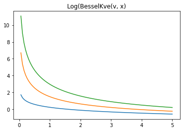
- 新增用於梯形積分的 tfp.math.trapz。
- 新增 tfp.math.log_bessel_kve。
- 將 no_pivot_ldl 新增至 experimental.linalg。
- 將 marginal_fn 引數新增至 GaussianProcess (請參閱 no_pivot_ldl)。
- 新增 tfp.math.atan_difference(x, y)
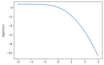
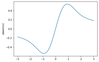
- 新增 tfp.math.erfcx、tfp.math.logerfc 和 tfp.math.logerfcx
- 新增用於 Dawson 積分的 tfp.math.dawsn。
- 新增 tfp.math.igammaincinv、tfp.math.igammacinv。
- 新增 tfp.math.sqrt1pm1。
- 新增 LogitNormal.stddev_approx 和 LogitNormal.variance_approx
- 新增用於 Owen's T 函數的 tfp.math.owens_t。
- 新增 bracket_root 方法，以自動初始化根搜尋的邊界。
- 新增 Chandrupatla 方法，以尋找純量函數的根。
統計
- tfp.stats.windowed_mean 有效率地計算視窗平均值。
- tfp.stats.windowed_variance 有效率且準確地計算視窗變異數。
- tfp.stats.cumulative_variance 有效率且準確地計算累積變異數。
- RunningCovariance 和朋友現在可以從範例張量初始化，而不僅僅是從明確的形狀和 dtype 初始化。
- 用於 RunningCentralMoments、RunningMean、RunningPotentialScaleReduction 的更簡潔 API。

Owen's T、Erfcx、Logerfc、Logerfcx、Dawson 函數

# Owen's T gives the probability that X > h, 0 < Y < a * X. Let's check that
# with random sampling.
h = np.array([1., 2.]).astype(np.float32)
a = np.array([10., 11.5]).astype(np.float32)
probs = tfp.math.owens_t(h, a)

x = tfd.Normal(0., 1.).sample(int(1e5), seed=(6, 245)).numpy()
y = tfd.Normal(0., 1.).sample(int(1e5), seed=(7, 245)).numpy()

true_values = (
    (x[..., np.newaxis] > h) &
    (0. < y[..., np.newaxis]) &
    (y[..., np.newaxis] < a * x[..., np.newaxis]))

print('Calculated values: {}'.format(
    np.count_nonzero(true_values, axis=0) / 1e5))

print('Expected values: {}'.format(probs))

Calculated values: [0.07896 0.01134]
Expected values: [0.07932763 0.01137507]

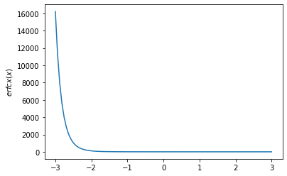
x = np.linspace(-3., 3., 100)
plt.plot(x, tfp.math.erfcx(x))
plt.ylabel('$erfcx(x)$')
plt.show()

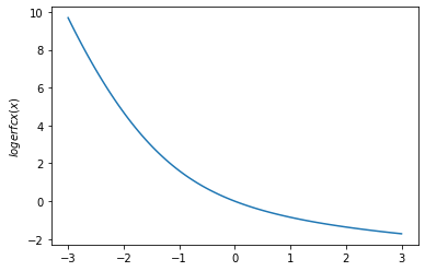
plt.plot(x, tfp.math.logerfcx(x))
plt.ylabel('$logerfcx(x)$')
plt.show()

plt.plot(x, tfp.math.logerfc(x))
plt.ylabel('$logerfc(x)$')
plt.show()

plt.plot(x, tfp.math.dawsn(x))
plt.ylabel('$dawsn(x)$')
plt.show()

png

igammainv / igammacinv

# Igammainv and Igammacinv are inverses to Igamma and Igammac

x = np.linspace(1., 10., 10)
y = tf.math.igamma(0.3, x)
x_prime = tfp.math.igammainv(0.3, y)
print('x: {}'.format(x))
print('igammainv(igamma(a, x)):\n {}'.format(x_prime))

y = tf.math.igammac(0.3, x)
x_prime = tfp.math.igammacinv(0.3, y)

print('\n')
print('x: {}'.format(x))
print('igammacinv(igammac(a, x)):\n {}'.format(x_prime))

x: [ 1.  2.  3.  4.  5.  6.  7.  8.  9. 10.]
igammainv(igamma(a, x)):
 [1.        1.9999992 3.000003  4.0000024 5.0000257 5.999887  7.0002484
 7.999243  8.99872   9.994673 ]


x: [ 1.  2.  3.  4.  5.  6.  7.  8.  9. 10.]
igammacinv(igammac(a, x)):
 [1.       2.       3.       4.       5.       6.       7.       8.000001

 9.       9.999999]

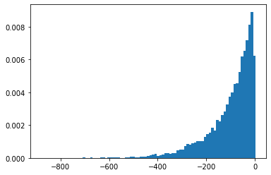
log-kve

x = np.linspace(0., 5., 100)
for v in [0.5, 2., 3]:
  plt.plot(x, tfp.math.log_bessel_kve(v, x).numpy())

plt.title('Log(BesselKve(v, x)')

Text(0.5, 1.0, 'Log(BesselKve(v, x)')

png

其他

STS
- 使用內部 tf.function 包裝加速 STS 預測和分解。
- 當只需要最後一步的結果時，新增選項以加速 LinearGaussianSSM 中的篩選。
- 具有聯合分佈的變異數推論：具有氡模型的範例筆記本。
- 新增實驗性支援，以將任何分佈轉換為預先調節雙射器。
新增 tfp.random.sanitize_seed。
新增 tfp.random.spherical_uniform。

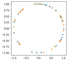
plt.figure(figsize=(4, 4))
seed = tfp.random.sanitize_seed(123)
seed1, seed2 = tfp.random.split_seed(seed)
samps = tfp.random.spherical_uniform([30], dimension=2, seed=seed1)
plt.scatter(*samps.numpy().T, marker='+')
samps = tfp.random.spherical_uniform([30], dimension=2, seed=seed2)
plt.scatter(*samps.numpy().T, marker='+');

png

TFP 版本說明筆記本 (0.13.0)

安裝與匯入

分佈 [核心數學]

BetaQuotient

DeterminantalPointProcess

SigmoidBeta

Zipf

NormalInverseGaussian

MatrixNormalLinearOperator

MatrixStudentTLinearOperator

分佈 [軟體/包裝函式]

Sharded

BatchBroadcast

Masked

雙射器

重組雙射器

Sharded

VI

VI/MAP/MLE

MCMC

init_near_unconstrained_zero、retry_init

視窗化自適應 HMC 和 NUTS 採樣器

數學、統計

Owen's T、Erfcx、Logerfc、Logerfcx、Dawson 函數

igammainv / igammacinv

log-kve

其他

`BetaQuotient`

`DeterminantalPointProcess`

`SigmoidBeta`

`NormalInverseGaussian`

`MatrixNormalLinearOperator`

`MatrixStudentTLinearOperator`

`Sharded`

`BatchBroadcast`

`Masked`

`Sharded`

`init_near_unconstrained_zero`、`retry_init`