from pprint import pprint
import matplotlib.pyplot as plt
import numpy as np
import seaborn as sns

import tensorflow as tf
import tf_keras

import tensorflow_probability as tfp

sns.reset_defaults()
#sns.set_style('whitegrid')
#sns.set_context('talk')
sns.set_context(context='talk',font_scale=0.7)

%matplotlib inline

tfd = tfp.distributions
加速運算!
在我們深入探討之前,請先確認我們在此示範中使用了 GPU。
若要執行此操作,請選取「執行階段」->「變更執行階段類型」->「硬體加速器」->「GPU」。
以下程式碼片段將驗證我們是否可以存取 GPU。
if tf.test.gpu_device_name() != '/device:GPU:0':
  print('WARNING: GPU device not found.')
else:
  print('SUCCESS: Found GPU: {}'.format(tf.test.gpu_device_name()))
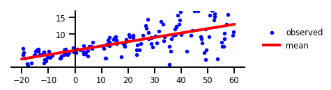
plt.figure(figsize=[6, 1.5]) # inches
plt.plot(x, y, 'b.', label='observed');
yhats = [model(x_tst) for _ in range(100)]
avgm = np.zeros_like(x_tst[..., 0])
for i, yhat in enumerate(yhats):
m = np.squeeze(yhat.mean())
s = np.squeeze(yhat.stddev())
if i < 15:
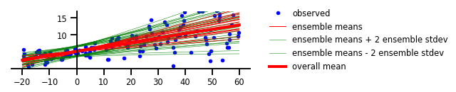
plt.plot(x_tst, m, 'r', label='ensemble means' if i == 0 else None, linewidth=1.)
plt.plot(x_tst, m + 2 * s, 'g', linewidth=0.5, label='ensemble means + 2 ensemble stdev' if i == 0 else None);
plt.plot(x_tst, m - 2 * s, 'g', linewidth=0.5, label='ensemble means - 2 ensemble stdev' if i == 0 else None);
avgm += m
plt.plot(x_tst, avgm/len(yhats), 'r', label='overall mean', linewidth=4)
plt.ylim(-0.,17);
plt.yticks(np.linspace(0, 15, 4)[1:]);
plt.xticks(np.linspace(*x_range, num=9));
ax=plt.gca();
ax.xaxis.set_ticks_position('bottom')
ax.yaxis.set_ticks_position('left')
ax.spines['left'].set_position(('data', 0))
ax.spines['top'].set_visible(False)
ax.spines['right'].set_visible(False)
#ax.spines['left'].set_smart_bounds(True)
#ax.spines['bottom'].set_smart_bounds(True)
plt.legend(loc='center left', fancybox=True, framealpha=0., bbox_to_anchor=(1.05, 0.5))
plt.savefig('/tmp/fig4.png', bbox_inches='tight', dpi=300)
案例 5:函數不確定性
自訂 PSD 核心
class RBFKernelFn(tf_keras.layers.Layer):
  def __init__(self, **kwargs):
    super(RBFKernelFn, self).__init__(**kwargs)
    dtype = kwargs.get('dtype', None)

    self._amplitude = self.add_variable(
            initializer=tf.constant_initializer(0),
            dtype=dtype,
            name='amplitude')

    self._length_scale = self.add_variable(
            initializer=tf.constant_initializer(0),
            dtype=dtype,
            name='length_scale')

  def call(self, x):
    # Never called -- this is just a layer so it can hold variables
    # in a way Keras understands.
    return x

  @property
  def kernel(self):
    return tfp.math.psd_kernels.ExponentiatedQuadratic(
      amplitude=tf.nn.softplus(0.1 * self._amplitude),
      length_scale=tf.nn.softplus(5. * self._length_scale)
    )
# For numeric stability, set the default floating-point dtype to float64
tf_keras.backend.set_floatx('float64')

# Build model.
num_inducing_points = 40
model = tf_keras.Sequential([
    tf_keras.layers.InputLayer(input_shape=[1]),
    tf_keras.layers.Dense(1, kernel_initializer='ones', use_bias=False),
    tfp.layers.VariationalGaussianProcess(
        num_inducing_points=num_inducing_points,
        kernel_provider=RBFKernelFn(),
        event_shape=[1],
        inducing_index_points_initializer=tf.constant_initializer(
            np.linspace(*x_range, num=num_inducing_points,
                        dtype=x.dtype)[..., np.newaxis]),
        unconstrained_observation_noise_variance_initializer=(
            tf.constant_initializer(np.array(0.54).astype(x.dtype))),
    ),
])

# Do inference.
batch_size = 32
loss = lambda y, rv_y: rv_y.variational_loss(
    y, kl_weight=np.array(batch_size, x.dtype) / x.shape[0])
model.compile(optimizer=tf_keras.optimizers.Adam(learning_rate=0.01), loss=loss)
model.fit(x, y, batch_size=batch_size, epochs=1000, verbose=False)

# Profit.
yhat = model(x_tst)
assert isinstance(yhat, tfd.Distribution)
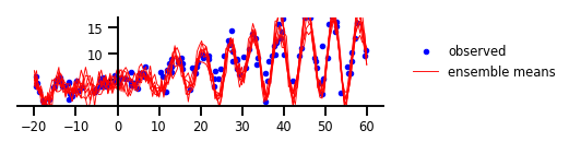
圖 5:函數不確定性
y, x, _ = load_dataset()

plt.figure(figsize=[6, 1.5])  # inches
plt.plot(x, y, 'b.', label='observed');

num_samples = 7
for i in range(num_samples):
  sample_ = yhat.sample().numpy()
  plt.plot(x_tst,
           sample_[..., 0].T,
           'r',
           linewidth=0.9,
           label='ensemble means' if i == 0 else None);

plt.ylim(-0.,17);
plt.yticks(np.linspace(0, 15, 4)[1:]);
plt.xticks(np.linspace(*x_range, num=9));

ax=plt.gca();
ax.xaxis.set_ticks_position('bottom')
ax.yaxis.set_ticks_position('left')
ax.spines['left'].set_position(('data', 0))
ax.spines['top'].set_visible(False)
ax.spines['right'].set_visible(False)
#ax.spines['left'].set_smart_bounds(True)
#ax.spines['bottom'].set_smart_bounds(True)
plt.legend(loc='center left', fancybox=True, framealpha=0., bbox_to_anchor=(1.05, 0.5))

plt.savefig('/tmp/fig5.png', bbox_inches='tight', dpi=300)

 在 GitHub 上檢視原始碼