
貝氏模型選擇
|
|
|
 在 GitHub 上檢視原始碼 在 GitHub 上檢視原始碼
|
|
匯入
import numpy as np
import tensorflow as tf
import tf_keras
import tensorflow_probability as tfp
from tensorflow_probability import distributions as tfd

from matplotlib import pylab as plt
%matplotlib inline
import scipy.stats
任務:多重變異點偵測
考慮一個變異點偵測任務:事件發生的速率隨時間變化,這是由產生資料的某些系統或程序的 (未觀察到) 狀態突然轉變所驅動。
例如,我們可能會觀察到如下所示的一系列計數
true_rates = [40, 3, 20, 50]
true_durations = [10, 20, 5, 35]

observed_counts = tf.concat(
    [tfd.Poisson(rate).sample(num_steps)
     for (rate, num_steps) in zip(true_rates, true_durations)], axis=0)

plt.plot(observed_counts)
[<matplotlib.lines.Line2D at 0x7f7589bdae10>]
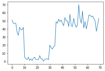
這些計數可以代表資料中心的故障次數、網頁的訪客人數、網路連結上的封包數等等。
請注意,僅從資料中並不明顯看出有多少個不同的系統狀態。您能分辨出三個切換點分別發生在哪裡嗎?
已知狀態數量
我們首先考慮 (可能不切實際的) 情況,即事先已知未觀察到的狀態數量。在這裡,我們假設我們知道有四個潛在狀態。
我們將此問題建模為切換 (非均勻) 卜瓦松過程:在每個時間點,發生的事件數量呈卜瓦松分佈,而事件的速率由未觀察到的系統狀態 \(z_t\) 決定
\[x_t \sim \text{Poisson}(\lambda_{z_t})\]
潛在狀態是離散的:\(z_t \in \{1, 2, 3, 4\}\),因此 \(\lambda = [\lambda_1, \lambda_2, \lambda_3, \lambda_4]\) 是一個簡單的向量,其中包含每個狀態的卜瓦松率。為了模擬狀態隨時間的演變,我們將定義一個簡單的轉移模型 \(p(z_t | z_{t-1})\):假設在每個步驟中,我們以機率 \(p\) 保持在先前的狀態,並以機率 \(1-p\) 均勻隨機地轉移到不同的狀態。初始狀態也是均勻隨機選擇的,因此我們有
\[ \begin{align*} z_1 &\sim \text{Categorical}\left(\left\{\frac{1}{4}, \frac{1}{4}, \frac{1}{4}, \frac{1}{4}\right\}\right)\\ z_t | z_{t-1} &\sim \text{Categorical}\left(\left\{\begin{array}{cc}p & \text{if } z_t = z_{t-1} \\ \frac{1-p}{4-1} & \text{otherwise}\end{array}\right\}\right) \end{align*}\]
這些假設對應於具有卜瓦松射出的 隱藏式馬可夫模型。我們可以使用 tfd.HiddenMarkovModel 在 TFP 中對其進行編碼。首先,我們定義轉移矩陣和初始狀態的均勻先驗
num_states = 4
initial_state_logits = tf.zeros([num_states]) # uniform distribution

daily_change_prob = 0.05
transition_probs = tf.fill([num_states, num_states],
                           daily_change_prob / (num_states - 1))
transition_probs = tf.linalg.set_diag(transition_probs,
                                      tf.fill([num_states],
                                              1 - daily_change_prob))

print("Initial state logits:\n{}".format(initial_state_logits))
print("Transition matrix:\n{}".format(transition_probs))
Initial state logits:
[0. 0. 0. 0.]
Transition matrix:
[[0.95       0.01666667 0.01666667 0.01666667]
 [0.01666667 0.95       0.01666667 0.01666667]
 [0.01666667 0.01666667 0.95       0.01666667]
 [0.01666667 0.01666667 0.01666667 0.95      ]]
接下來,我們建立 tfd.HiddenMarkovModel 分佈,使用可訓練變數來表示與每個系統狀態相關聯的速率。我們在對數空間中參數化速率,以確保它們是正值。
# Define variable to represent the unknown log rates.
trainable_log_rates = tf.Variable(
  tf.math.log(tf.reduce_mean(observed_counts)) +
  tf.random.stateless_normal([num_states], seed=(42, 42)),
  name='log_rates')

hmm = tfd.HiddenMarkovModel(
  initial_distribution=tfd.Categorical(
      logits=initial_state_logits),
  transition_distribution=tfd.Categorical(probs=transition_probs),
  observation_distribution=tfd.Poisson(log_rate=trainable_log_rates),
  num_steps=len(observed_counts))
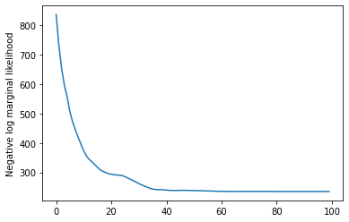
最後,我們定義模型的總對數密度,包括速率的弱資訊性對數常態先驗,並執行最佳化工具來計算觀察到的計數資料的 最大後驗 (MAP) 擬合。
rate_prior = tfd.LogNormal(5, 5)

def log_prob():
 return (tf.reduce_sum(rate_prior.log_prob(tf.math.exp(trainable_log_rates))) +
         hmm.log_prob(observed_counts))

losses = tfp.math.minimize(
    lambda: -log_prob(),
    optimizer=tf_keras.optimizers.Adam(learning_rate=0.1),
    num_steps=100)
plt.plot(losses)
plt.ylabel('Negative log marginal likelihood')
Text(0, 0.5, 'Negative log marginal likelihood')
rates = tf.exp(trainable_log_rates)
print("Inferred rates: {}".format(rates))
print("True rates: {}".format(true_rates))
Inferred rates: [ 2.8302798 49.58499   41.928307  17.35112  ]
True rates: [40, 3, 20, 50]
成功了!請注意,此模型中的潛在狀態僅可識別到置換,因此我們恢復的速率順序不同,並且有一些雜訊,但總體而言,它們非常吻合。
恢復狀態軌跡
現在我們已經擬合模型,我們可能想要重建模型認為系統在每個時間步處於哪個狀態。
這是一項後驗推論任務:給定觀察到的計數 \(x_{1:T}\) 和模型參數 (速率) \(\lambda\),我們想要推斷離散潛在變數的序列,遵循後驗分佈 \(p(z_{1:T} | x_{1:T}, \lambda)\)。在隱藏式馬可夫模型中,我們可以使用標準訊息傳遞演算法有效率地計算此分佈的邊際分佈和其他屬性。特別是,posterior_marginals 方法將有效率地計算 (使用 前向-後向演算法) 邊際機率分佈 \(p(Z_t = z_t | x_{1:T})\),其在每個時間步 \(t\) 處,針對離散潛在狀態 \(Z_t\)。
# Runs forward-backward algorithm to compute marginal posteriors.
posterior_dists = hmm.posterior_marginals(observed_counts)
posterior_probs = posterior_dists.probs_parameter().numpy()
繪製後驗機率,我們恢復了模型對資料的「解釋」:每個狀態在哪些時間點處於活動狀態?
def plot_state_posterior(ax, state_posterior_probs, title):
  ln1 = ax.plot(state_posterior_probs, c='blue', lw=3, label='p(state | counts)')
  ax.set_ylim(0., 1.1)
  ax.set_ylabel('posterior probability')
  ax2 = ax.twinx()
  ln2 = ax2.plot(observed_counts, c='black', alpha=0.3, label='observed counts')
  ax2.set_title(title)
  ax2.set_xlabel("time")
  lns = ln1+ln2
  labs = [l.get_label() for l in lns]
  ax.legend(lns, labs, loc=4)
  ax.grid(True, color='white')
  ax2.grid(False)

fig = plt.figure(figsize=(10, 10))
plot_state_posterior(fig.add_subplot(2, 2, 1),
                     posterior_probs[:, 0],
                     title="state 0 (rate {:.2f})".format(rates[0]))
plot_state_posterior(fig.add_subplot(2, 2, 2),
                     posterior_probs[:, 1],
                     title="state 1 (rate {:.2f})".format(rates[1]))
plot_state_posterior(fig.add_subplot(2, 2, 3),
                     posterior_probs[:, 2],
                     title="state 2 (rate {:.2f})".format(rates[2]))
plot_state_posterior(fig.add_subplot(2, 2, 4),
                     posterior_probs[:, 3],
                     title="state 3 (rate {:.2f})".format(rates[3]))
plt.tight_layout()
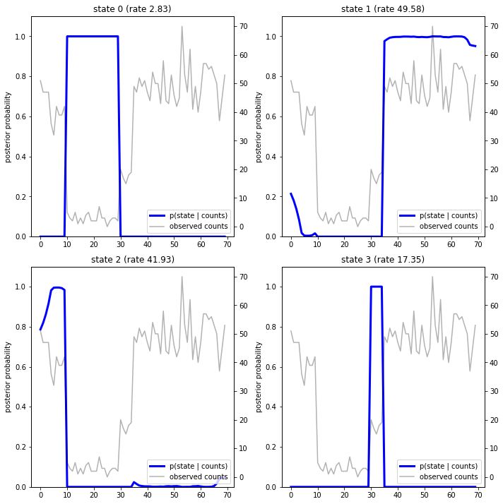
在這個 (簡單的) 案例中,我們看到模型通常相當有信心:在大多數時間步中,它基本上將所有機率質量分配給四個狀態中的一個。幸運的是,這些解釋看起來很合理!
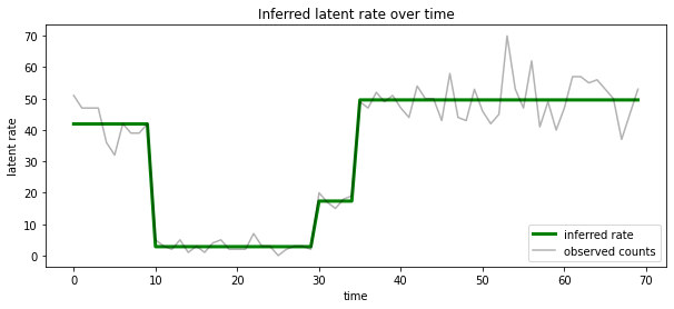
我們也可以根據與每個時間步中最可能的潛在狀態相關聯的速率來視覺化此後驗,將機率後驗濃縮為單一解釋
most_probable_states = hmm.posterior_mode(observed_counts)
most_probable_rates = tf.gather(rates, most_probable_states)
fig = plt.figure(figsize=(10, 4))
ax = fig.add_subplot(1, 1, 1)
ax.plot(most_probable_rates, c='green', lw=3, label='inferred rate')
ax.plot(observed_counts, c='black', alpha=0.3, label='observed counts')
ax.set_ylabel("latent rate")
ax.set_xlabel("time")
ax.set_title("Inferred latent rate over time")
ax.legend(loc=4)
<matplotlib.legend.Legend at 0x7f75849e70f0>
未知狀態數量
在實際問題中,我們可能不知道我們正在建模的系統中「真實」狀態的數量。這可能不總是需要擔心:如果您特別不關心未知狀態的身分,您可以只執行一個狀態數量多於您知道模型需要的模型,並學習 (類似於) 一堆實際狀態的重複副本。但讓我們假設您確實關心推斷「真實」潛在狀態的數量。
我們可以將其視為 貝氏模型選擇 的案例:我們有一組候選模型,每個模型都有不同數量的潛在狀態,我們想要選擇最有可能產生觀察資料的模型。為此,我們計算每個模型下資料的邊際概似 (我們也可以在模型本身上新增先驗,但在本次分析中這不是必要的;貝氏奧卡姆剃刀 證明足以編碼對較簡單模型的偏好)。
遺憾的是,真正的邊際概似 (其對離散狀態 \(z_{1:T}\) 和 (速率參數向量) \(\lambda\) 進行積分) \(p(x_{1:T}) = \int p(x_{1:T}, z_{1:T}, \lambda) dz d\lambda,\) 對於此模型來說是難以處理的。為了方便起見,我們將使用所謂的「經驗貝氏」或「II 型最大概似」估計來近似它:我們將最佳化其值,而不是完全積分出與每個系統狀態相關聯的 (未知) 速率參數 \(\lambda\)
\[\tilde{p}(x_{1:T}) = \max_\lambda \int p(x_{1:T}, z_{1:T}, \lambda) dz\]
這種近似可能會過度擬合,也就是說,它會比真正的邊際概似更偏好更複雜的模型。我們可以考慮更忠實的近似,例如,最佳化變分下限,或使用蒙地卡羅估計器 (例如 退火重要性取樣);這些 (遺憾地) 超出了本筆記本的範圍。(如需更多關於貝氏模型選擇和近似的資訊,優秀著作 Machine Learning: a Probabilistic Perspective 的第 7 章是一個很好的參考。)
原則上,我們可以透過使用不同的 num_states 值多次重新執行上述最佳化來進行模型比較,但這會是大量的工作。在這裡,我們將展示如何使用 TFP 的 batch_shape 機制進行向量化,以平行處理多個模型。
轉移矩陣和初始狀態先驗:現在我們將建構一批轉移矩陣和先驗 logits,而不是建構單一模型描述,每個候選模型最多為 max_num_states。為了方便批次處理,我們需要確保所有計算都具有相同的「形狀」:這必須對應於我們將擬合的最大模型的維度。為了處理較小的模型,我們可以將它們的描述「嵌入」到狀態空間的最頂層維度中,有效地將剩餘維度視為從未使用過的虛擬狀態。
max_num_states = 10

def build_latent_state(num_states, max_num_states, daily_change_prob=0.05):

  # Give probability exp(-100) ~= 0 to states outside of the current model.
  active_states_mask = tf.concat([tf.ones([num_states]),
                                  tf.zeros([max_num_states - num_states])],
                                 axis=0)
  initial_state_logits = -100. * (1 - active_states_mask)

  # Build a transition matrix that transitions only within the current
  # `num_states` states.
  transition_probs = tf.fill([num_states, num_states],
                             0. if num_states == 1
                             else daily_change_prob / (num_states - 1))
  padded_transition_probs = tf.eye(max_num_states) + tf.pad(
      tf.linalg.set_diag(transition_probs,
                         tf.fill([num_states], - daily_change_prob)),
      paddings=[(0, max_num_states - num_states),
                (0, max_num_states - num_states)])

  return initial_state_logits, padded_transition_probs

# For each candidate model, build the initial state prior and transition matrix.
batch_initial_state_logits = []
batch_transition_probs = []
for num_states in range(1, max_num_states+1):
  initial_state_logits, transition_probs = build_latent_state(
      num_states=num_states,
      max_num_states=max_num_states)
  batch_initial_state_logits.append(initial_state_logits)
  batch_transition_probs.append(transition_probs)

batch_initial_state_logits = tf.stack(batch_initial_state_logits)
batch_transition_probs = tf.stack(batch_transition_probs)
print("Shape of initial_state_logits: {}".format(batch_initial_state_logits.shape))
print("Shape of transition probs: {}".format(batch_transition_probs.shape))
print("Example initial state logits for num_states==3:\n{}".format(batch_initial_state_logits[2, :]))
print("Example transition_probs for num_states==3:\n{}".format(batch_transition_probs[2, :, :]))
Shape of initial_state_logits: (10, 10)
Shape of transition probs: (10, 10, 10)
Example initial state logits for num_states==3:
[  -0.   -0.   -0. -100. -100. -100. -100. -100. -100. -100.]
Example transition_probs for num_states==3:
[[0.95  0.025 0.025 0.    0.    0.    0.    0.    0.    0.   ]
 [0.025 0.95  0.025 0.    0.    0.    0.    0.    0.    0.   ]
 [0.025 0.025 0.95  0.    0.    0.    0.    0.    0.    0.   ]
 [0.    0.    0.    1.    0.    0.    0.    0.    0.    0.   ]
 [0.    0.    0.    0.    1.    0.    0.    0.    0.    0.   ]
 [0.    0.    0.    0.    0.    1.    0.    0.    0.    0.   ]
 [0.    0.    0.    0.    0.    0.    1.    0.    0.    0.   ]
 [0.    0.    0.    0.    0.    0.    0.    1.    0.    0.   ]
 [0.    0.    0.    0.    0.    0.    0.    0.    1.    0.   ]
 [0.    0.    0.    0.    0.    0.    0.    0.    0.    1.   ]]
現在我們以與上述類似的方式進行。這次我們將在 trainable_rates 中使用額外的批次維度,以分別擬合每個考慮模型的速率。
trainable_log_rates = tf.Variable(
    tf.fill([batch_initial_state_logits.shape[0], max_num_states],
            tf.math.log(tf.reduce_mean(observed_counts))) +
     tf.random.stateless_normal([1, max_num_states], seed=(42, 42)),
     name='log_rates')

hmm = tfd.HiddenMarkovModel(
  initial_distribution=tfd.Categorical(
      logits=batch_initial_state_logits),
  transition_distribution=tfd.Categorical(probs=batch_transition_probs),
  observation_distribution=tfd.Poisson(log_rate=trainable_log_rates),
  num_steps=len(observed_counts))
print("Defined HMM with batch shape: {}".format(hmm.batch_shape))
Defined HMM with batch shape: (10,)
在計算總對數機率時,我們謹慎地僅對每個模型元件實際使用的速率的先驗求和
rate_prior = tfd.LogNormal(5, 5)

def log_prob():
  prior_lps = rate_prior.log_prob(tf.math.exp(trainable_log_rates))
  prior_lp = tf.stack(
      [tf.reduce_sum(prior_lps[i, :i+1]) for i in range(max_num_states)])
  return prior_lp + hmm.log_prob(observed_counts)
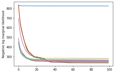
現在我們最佳化我們建構的批次目標,同時擬合所有候選模型
losses = tfp.math.minimize(
    lambda: -log_prob(),
    optimizer=tf_keras.optimizers.Adam(0.1),
    num_steps=100)
plt.plot(losses)
plt.ylabel('Negative log marginal likelihood')
Text(0, 0.5, 'Negative log marginal likelihood')
num_states = np.arange(1, max_num_states+1)
plt.plot(num_states, -losses[-1])
plt.ylim([-400, -200])
plt.ylabel("marginal likelihood $\\tilde{p}(x)$")
plt.xlabel("number of latent states")
plt.title("Model selection on latent states")
Text(0.5, 1.0, 'Model selection on latent states')

檢查概似,我們看到 (近似) 邊際概似傾向於偏好三狀態模型。這似乎很合理——「真實」模型有四個狀態,但僅從資料來看,很難排除三狀態解釋。
我們也可以提取每個候選模型的擬合速率
rates = tf.exp(trainable_log_rates)
for i, learned_model_rates in enumerate(rates):
  print("rates for {}-state model: {}".format(i+1, learned_model_rates[:i+1]))
rates for 1-state model: [32.968506]
rates for 2-state model: [ 5.789209 47.948917]
rates for 3-state model: [ 2.841977 48.057507 17.958897]
rates for 4-state model: [ 2.8302798 49.585037  41.928406  17.351114 ]
rates for 5-state model: [17.399694  77.83679   41.975216  49.62771    2.8256145]
rates for 6-state model: [41.63677   77.20768   49.570934  49.557076  17.630419   2.8713436]
rates for 7-state model: [41.711704  76.405945  49.581184  49.561283  17.451889   2.8722699
 17.43608  ]
rates for 8-state model: [41.771793 75.41323  49.568714 49.591846 17.2523   17.247969 17.231388
  2.830598]
rates for 9-state model: [41.83378   74.50916   49.619488  49.622494   2.8369408 17.254414
 17.21532    2.5904858 17.252514 ]
rates for 10-state model: [4.1886074e+01 7.3912338e+01 4.1940136e+01 4.9652588e+01 2.8485537e+00
 1.7433832e+01 6.7564294e-02 1.9590002e+00 1.7430998e+01 7.8838937e-02]
並繪製每個模型為資料提供的解釋
most_probable_states = hmm.posterior_mode(observed_counts)
fig = plt.figure(figsize=(14, 12))
for i, learned_model_rates in enumerate(rates):
  ax = fig.add_subplot(4, 3, i+1)
  ax.plot(tf.gather(learned_model_rates, most_probable_states[i]), c='green', lw=3, label='inferred rate')
  ax.plot(observed_counts, c='black', alpha=0.3, label='observed counts')
  ax.set_ylabel("latent rate")
  ax.set_xlabel("time")
  ax.set_title("{}-state model".format(i+1))
  ax.legend(loc=4)
plt.tight_layout()
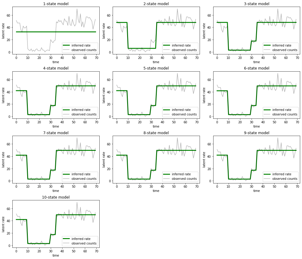
很容易看出,單狀態、雙狀態和 (更微妙的) 三狀態模型如何提供不足的解釋。有趣的是,所有高於四狀態的模型都提供了基本相同的解釋!這可能是因為我們的「資料」相對乾淨,幾乎沒有替代解釋的空間;在更混亂的真實世界資料中,我們預期更高容量的模型會為資料提供逐漸更好的擬合,並在改進的擬合被模型複雜性超過時達到某個權衡點。
擴充功能
本筆記本中的模型可以透過多種方式直接擴充。例如
- 允許潛在狀態具有不同的機率 (某些狀態可能常見與稀有)
- 允許潛在狀態之間進行非均勻轉移 (例如,學習到機器崩潰通常接著系統重新啟動,而系統重新啟動通常接著一段良好的效能期等等)
- 其他射出模型,例如
NegativeBinomial以模擬計數資料中不同的分散性,或連續分佈,例如Normal用於實值資料。