貝氏建模與聯合分佈

在 TensorFlow.org 上檢視

在 Google Colab 中執行

在 GitHub 上檢視原始碼

下載筆記本

JointDistributionSequential 是一種新推出的類別，類似於分佈，讓使用者能夠快速建立貝氏模型的原型。它讓您可以將多個分佈串連在一起，並使用 lambda 函數來引入依賴關係。此類別旨在建構中小型貝氏模型，包括許多常用的模型，例如 GLM、混合效應模型、混合模型等等。它啟用了貝氏工作流程所需的所有必要功能：先驗預測抽樣，它可以插入另一個更大的貝氏圖形模型或神經網路。在這個 Colab 中，我們將展示如何使用 JointDistributionSequential 來實現您日常的貝氏工作流程

依賴關係與先決條件

# We will be using ArviZ, a multi-backend Bayesian diagnosis and plotting library
pip3 install -q git+git://github.com/arviz-devs/arviz.git

匯入與設定

from pprint import pprint
import matplotlib.pyplot as plt
import numpy as np
import seaborn as sns
import pandas as pd
import arviz as az

import tensorflow as tf
import tf_keras
import tensorflow_probability as tfp

sns.reset_defaults()
#sns.set_style('whitegrid')
#sns.set_context('talk')
sns.set_context(context='talk',font_scale=0.7)

%config InlineBackend.figure_format = 'retina'
%matplotlib inline

tfd = tfp.distributions
tfb = tfp.bijectors

dtype = tf.float64

加速！

在我們深入探討之前，我們先確認一下這個示範使用了 GPU。

若要執行此操作，請依序選取「執行階段」->「變更執行階段類型」->「硬體加速器」->「GPU」。

以下程式碼片段將驗證我們是否可以使用 GPU。

if tf.test.gpu_device_name() != '/device:GPU:0':
  print('WARNING: GPU device not found.')
else:
  print('SUCCESS: Found GPU: {}'.format(tf.test.gpu_device_name()))

SUCCESS: Found GPU: /device:GPU:0

JointDistribution

注意事項：當您只有簡單的模型時，這個分佈類別非常有用。「簡單」指的是鏈狀圖；雖然此方法在技術上適用於任何單一節點度數最多為 255 的 PGM（因為 Python 函數最多可以有這麼多個引數）。

基本概念是讓使用者指定一個可調用物件 (callable) 清單，每個物件都會產生一個 tfp.Distribution 執行個體，PGM 中的每個頂點各有一個執行個體。可調用物件的引數最多會與其在清單中的索引一樣多。（為了使用者方便起見，引數會以與建立順序相反的順序傳遞。）在內部，我們會透過將每個先前 RV 的值傳遞到每個可調用物件中來「走訪圖形」。這樣做，我們便實作了[機率的鏈鎖法則](https://en.wikipedia.org/wiki/Chainrule(probability%29#More_than_two_random_variables): \(p(\{x\}_i^d)=\prod_i^d p(x_i|x_{<i})\)。

這個概念非常簡單，即使以 Python 程式碼來看也是如此。以下是重點

# The chain rule of probability, manifest as Python code.
def log_prob(rvs, xs):
  # xs[:i] is rv[i]'s markov blanket. `[::-1]` just reverses the list.
  return sum(rv(*xs[i-1::-1]).log_prob(xs[i])
             for i, rv in enumerate(rvs))

您可以在 JointDistributionSequential 的文件字串中找到更多資訊，但重點是您傳遞分佈清單來初始化類別，如果清單中的某些分佈依賴於另一個上游分佈/變數的輸出，您只需使用 lambda 函數將其包裝起來。現在讓我們看看它在實際運作中的情況！

(穩健) 線性迴歸

出自 PyMC3 文件 GLM：使用離群值偵測的穩健迴歸

取得資料

dfhogg = pd.DataFrame(np.array([[1, 201, 592, 61, 9, -0.84],
                                 [2, 244, 401, 25, 4, 0.31],
                                 [3, 47, 583, 38, 11, 0.64],
                                 [4, 287, 402, 15, 7, -0.27],
                                 [5, 203, 495, 21, 5, -0.33],
                                 [6, 58, 173, 15, 9, 0.67],
                                 [7, 210, 479, 27, 4, -0.02],
                                 [8, 202, 504, 14, 4, -0.05],
                                 [9, 198, 510, 30, 11, -0.84],
                                 [10, 158, 416, 16, 7, -0.69],
                                 [11, 165, 393, 14, 5, 0.30],
                                 [12, 201, 442, 25, 5, -0.46],
                                 [13, 157, 317, 52, 5, -0.03],
                                 [14, 131, 311, 16, 6, 0.50],
                                 [15, 166, 400, 34, 6, 0.73],
                                 [16, 160, 337, 31, 5, -0.52],
                                 [17, 186, 423, 42, 9, 0.90],
                                 [18, 125, 334, 26, 8, 0.40],
                                 [19, 218, 533, 16, 6, -0.78],
                                 [20, 146, 344, 22, 5, -0.56]]),
                   columns=['id','x','y','sigma_y','sigma_x','rho_xy'])


## for convenience zero-base the 'id' and use as index
dfhogg['id'] = dfhogg['id'] - 1
dfhogg.set_index('id', inplace=True)

## standardize (mean center and divide by 1 sd)
dfhoggs = (dfhogg[['x','y']] - dfhogg[['x','y']].mean(0)) / dfhogg[['x','y']].std(0)
dfhoggs['sigma_y'] = dfhogg['sigma_y'] / dfhogg['y'].std(0)
dfhoggs['sigma_x'] = dfhogg['sigma_x'] / dfhogg['x'].std(0)

def plot_hoggs(dfhoggs):
  ## create xlims ylims for plotting
  xlims = (dfhoggs['x'].min() - np.ptp(dfhoggs['x'])/5,
           dfhoggs['x'].max() + np.ptp(dfhoggs['x'])/5)
  ylims = (dfhoggs['y'].min() - np.ptp(dfhoggs['y'])/5,
           dfhoggs['y'].max() + np.ptp(dfhoggs['y'])/5)

  ## scatterplot the standardized data
  g = sns.FacetGrid(dfhoggs, size=8)
  _ = g.map(plt.errorbar, 'x', 'y', 'sigma_y', 'sigma_x', marker="o", ls='')
  _ = g.axes[0][0].set_ylim(ylims)
  _ = g.axes[0][0].set_xlim(xlims)

  plt.subplots_adjust(top=0.92)
  _ = g.fig.suptitle('Scatterplot of Hogg 2010 dataset after standardization', fontsize=16)
  return g, xlims, ylims

g = plot_hoggs(dfhoggs)

/usr/local/lib/python3.6/dist-packages/numpy/core/fromnumeric.py:2495: FutureWarning: Method .ptp is deprecated and will be removed in a future version. Use numpy.ptp instead.
  return ptp(axis=axis, out=out, **kwargs)
/usr/local/lib/python3.6/dist-packages/seaborn/axisgrid.py:230: UserWarning: The `size` paramter has been renamed to `height`; please update your code.
  warnings.warn(msg, UserWarning)

X_np = dfhoggs['x'].values
sigma_y_np = dfhoggs['sigma_y'].values
Y_np = dfhoggs['y'].values

傳統 OLS 模型

現在，讓我們設定一個線性模型，一個簡單的截距 + 斜率迴歸問題

mdl_ols = tfd.JointDistributionSequential([
    # b0 ~ Normal(0, 1)
    tfd.Normal(loc=tf.cast(0, dtype), scale=1.),
    # b1 ~ Normal(0, 1)
    tfd.Normal(loc=tf.cast(0, dtype), scale=1.),
    # x ~ Normal(b0+b1*X, 1)
    lambda b1, b0: tfd.Normal(
      # Parameter transformation
      loc=b0 + b1*X_np,
      scale=sigma_y_np)
])

然後您可以檢查模型的圖形，以查看依賴關係。請注意，x 保留為最後一個節點的名稱，您不能在 JointDistributionSequential 模型中將其用作 lambda 引數。

mdl_ols.resolve_graph()

(('b0', ()), ('b1', ()), ('x', ('b1', 'b0')))

從模型中抽樣非常簡單

mdl_ols.sample()

[<tf.Tensor: shape=(), dtype=float64, numpy=-0.50225804634794>,
 <tf.Tensor: shape=(), dtype=float64, numpy=0.682740126293564>,
 <tf.Tensor: shape=(20,), dtype=float64, numpy=
 array([-0.33051382,  0.71443618, -1.91085683,  0.89371173, -0.45060957,
        -1.80448758, -0.21357082,  0.07891058, -0.20689721, -0.62690385,
        -0.55225748, -0.11446535, -0.66624497, -0.86913291, -0.93605552,
        -0.83965336, -0.70988597, -0.95813437,  0.15884761, -0.31113434])>]

...這會產生 tf.Tensor 的清單。您可以立即將其插入 log_prob 函數中，以計算模型的 log_prob

prior_predictive_samples = mdl_ols.sample()
mdl_ols.log_prob(prior_predictive_samples)

<tf.Tensor: shape=(20,), dtype=float64, numpy=
array([-4.97502846, -3.98544303, -4.37514505, -3.46933487, -3.80688125,
       -3.42907525, -4.03263074, -3.3646366 , -4.70370938, -4.36178501,
       -3.47823735, -3.94641662, -5.76906319, -4.0944128 , -4.39310708,
       -4.47713894, -4.46307881, -3.98802372, -3.83027747, -4.64777082])>

嗯，這裡似乎不太對勁：我們應該得到純量 log_prob！事實上，我們可以進一步檢查是否有問題，方法是呼叫 .log_prob_parts，它會提供圖形模型中每個節點的 log_prob

mdl_ols.log_prob_parts(prior_predictive_samples)

[<tf.Tensor: shape=(), dtype=float64, numpy=-0.9699239562734849>,
 <tf.Tensor: shape=(), dtype=float64, numpy=-3.459364167569284>,
 <tf.Tensor: shape=(20,), dtype=float64, numpy=
 array([-0.54574034,  0.4438451 ,  0.05414307,  0.95995326,  0.62240687,
         1.00021288,  0.39665739,  1.06465152, -0.27442125,  0.06750311,
         0.95105078,  0.4828715 , -1.33977506,  0.33487533,  0.03618104,
        -0.04785082, -0.03379069,  0.4412644 ,  0.59901066, -0.2184827 ])>]

...結果發現最後一個節點沒有沿著 i.i.d. 維度/軸進行 reduce_sum！當我們進行總和時，前兩個變數因此被錯誤地廣播。

這裡的技巧是使用 tfd.Independent 重新解釋批次形狀（以便其餘軸會正確縮減）

mdl_ols_ = tfd.JointDistributionSequential([
    # b0
    tfd.Normal(loc=tf.cast(0, dtype), scale=1.),
    # b1
    tfd.Normal(loc=tf.cast(0, dtype), scale=1.),
    # likelihood
    #   Using Independent to ensure the log_prob is not incorrectly broadcasted
    lambda b1, b0: tfd.Independent(
        tfd.Normal(
            # Parameter transformation
            # b1 shape: (batch_shape), X shape (num_obs): we want result to have
            # shape (batch_shape, num_obs)
            loc=b0 + b1*X_np,
            scale=sigma_y_np),
        reinterpreted_batch_ndims=1
    ),
])

現在，讓我們檢查模型的最後一個節點/分佈，您可以看到事件形狀現在已正確解釋。請注意，可能需要一些試錯才能讓 reinterpreted_batch_ndims 正確，但您隨時可以輕鬆列印分佈或抽樣張量來再次檢查形狀！

print(mdl_ols_.sample_distributions()[0][-1])
print(mdl_ols.sample_distributions()[0][-1])

tfp.distributions.Independent("JointDistributionSequential_sample_distributions_IndependentJointDistributionSequential_sample_distributions_Normal", batch_shape=[], event_shape=[20], dtype=float64)
tfp.distributions.Normal("JointDistributionSequential_sample_distributions_Normal", batch_shape=[20], event_shape=[], dtype=float64)

prior_predictive_samples = mdl_ols_.sample()
mdl_ols_.log_prob(prior_predictive_samples)  # <== Getting a scalar correctly

<tf.Tensor: shape=(), dtype=float64, numpy=-2.543425661013286>

其他 JointDistribution* API

mdl_ols_named = tfd.JointDistributionNamed(dict(
    likelihood = lambda b0, b1: tfd.Independent(
        tfd.Normal(
            loc=b0 + b1*X_np,
            scale=sigma_y_np),
        reinterpreted_batch_ndims=1
    ),
    b0         = tfd.Normal(loc=tf.cast(0, dtype), scale=1.),
    b1         = tfd.Normal(loc=tf.cast(0, dtype), scale=1.),
))

mdl_ols_named.log_prob(mdl_ols_named.sample())

<tf.Tensor: shape=(), dtype=float64, numpy=-5.99620966071338>

mdl_ols_named.sample()  # output is a dictionary

{'b0': <tf.Tensor: shape=(), dtype=float64, numpy=0.26364058399428225>,
 'b1': <tf.Tensor: shape=(), dtype=float64, numpy=-0.27209402374432207>,
 'likelihood': <tf.Tensor: shape=(20,), dtype=float64, numpy=
 array([ 0.6482155 , -0.39314108,  0.62744764, -0.24587987, -0.20544617,
         1.01465392, -0.04705611, -0.16618702,  0.36410134,  0.3943299 ,
         0.36455291, -0.27822219, -0.24423928,  0.24599518,  0.82731092,
        -0.21983033,  0.56753169,  0.32830481, -0.15713064,  0.23336351])>}

Root = tfd.JointDistributionCoroutine.Root  # Convenient alias.
def model():
  b1 = yield Root(tfd.Normal(loc=tf.cast(0, dtype), scale=1.))
  b0 = yield Root(tfd.Normal(loc=tf.cast(0, dtype), scale=1.))
  yhat = b0 + b1*X_np
  likelihood = yield tfd.Independent(
        tfd.Normal(loc=yhat, scale=sigma_y_np),
        reinterpreted_batch_ndims=1
    )

mdl_ols_coroutine = tfd.JointDistributionCoroutine(model)
mdl_ols_coroutine.log_prob(mdl_ols_coroutine.sample())

<tf.Tensor: shape=(), dtype=float64, numpy=-4.566678123520463>

mdl_ols_coroutine.sample()  # output is a tuple

(<tf.Tensor: shape=(), dtype=float64, numpy=0.06811002171170354>,
 <tf.Tensor: shape=(), dtype=float64, numpy=-0.37477064754116807>,
 <tf.Tensor: shape=(20,), dtype=float64, numpy=
 array([-0.91615096, -0.20244718, -0.47840159, -0.26632479, -0.60441105,
        -0.48977789, -0.32422329, -0.44019322, -0.17072643, -0.20666025,
        -0.55932191, -0.40801868, -0.66893181, -0.24134135, -0.50403536,
        -0.51788596, -0.90071876, -0.47382338, -0.34821655, -0.38559724])>)

MLE

現在我們可以進行推論了！您可以使用最佳化工具來尋找最大概似估計。

定義一些輔助函數

# bfgs and lbfgs currently requries a function that returns both the value and
# gradient re the input.
import functools

def _make_val_and_grad_fn(value_fn):
  @functools.wraps(value_fn)
  def val_and_grad(x):
    return tfp.math.value_and_gradient(value_fn, x)
  return val_and_grad

# Map a list of tensors (e.g., output from JDSeq.sample([...])) to a single tensor
# modify from tfd.Blockwise
from tensorflow_probability.python.internal import dtype_util
from tensorflow_probability.python.internal import prefer_static as ps
from tensorflow_probability.python.internal import tensorshape_util

class Mapper:
  """Basically, this is a bijector without log-jacobian correction."""
  def __init__(self, list_of_tensors, list_of_bijectors, event_shape):
    self.dtype = dtype_util.common_dtype(
        list_of_tensors, dtype_hint=tf.float32)
    self.list_of_tensors = list_of_tensors
    self.bijectors = list_of_bijectors
    self.event_shape = event_shape

  def flatten_and_concat(self, list_of_tensors):
    def _reshape_map_part(part, event_shape, bijector):
      part = tf.cast(bijector.inverse(part), self.dtype)
      static_rank = tf.get_static_value(ps.rank_from_shape(event_shape))
      if static_rank == 1:
        return part
      new_shape = ps.concat([
          ps.shape(part)[:ps.size(ps.shape(part)) - ps.size(event_shape)], 
          [-1]
      ], axis=-1)
      return tf.reshape(part, ps.cast(new_shape, tf.int32))

    x = tf.nest.map_structure(_reshape_map_part,
                              list_of_tensors,
                              self.event_shape,
                              self.bijectors)
    return tf.concat(tf.nest.flatten(x), axis=-1)

  def split_and_reshape(self, x):
    assertions = []
    message = 'Input must have at least one dimension.'
    if tensorshape_util.rank(x.shape) is not None:
      if tensorshape_util.rank(x.shape) == 0:
        raise ValueError(message)
    else:
      assertions.append(assert_util.assert_rank_at_least(x, 1, message=message))
    with tf.control_dependencies(assertions):
      splits = [
          tf.cast(ps.maximum(1, ps.reduce_prod(s)), tf.int32)
          for s in tf.nest.flatten(self.event_shape)
      ]
      x = tf.nest.pack_sequence_as(
          self.event_shape, tf.split(x, splits, axis=-1))
      def _reshape_map_part(part, part_org, event_shape, bijector):
        part = tf.cast(bijector.forward(part), part_org.dtype)
        static_rank = tf.get_static_value(ps.rank_from_shape(event_shape))
        if static_rank == 1:
          return part
        new_shape = ps.concat([ps.shape(part)[:-1], event_shape], axis=-1)
        return tf.reshape(part, ps.cast(new_shape, tf.int32))

      x = tf.nest.map_structure(_reshape_map_part,
                                x, 
                                self.list_of_tensors,
                                self.event_shape,
                                self.bijectors)
    return x

mapper = Mapper(mdl_ols_.sample()[:-1],
                [tfb.Identity(), tfb.Identity()],
                mdl_ols_.event_shape[:-1])

# mapper.split_and_reshape(mapper.flatten_and_concat(mdl_ols_.sample()[:-1]))

@_make_val_and_grad_fn
def neg_log_likelihood(x):
  # Generate a function closure so that we are computing the log_prob
  # conditioned on the observed data. Note also that tfp.optimizer.* takes a 
  # single tensor as input.
  return -mdl_ols_.log_prob(mapper.split_and_reshape(x) + [Y_np])

lbfgs_results = tfp.optimizer.lbfgs_minimize(
    neg_log_likelihood,
    initial_position=tf.zeros(2, dtype=dtype),
    tolerance=1e-20,
    x_tolerance=1e-8
)

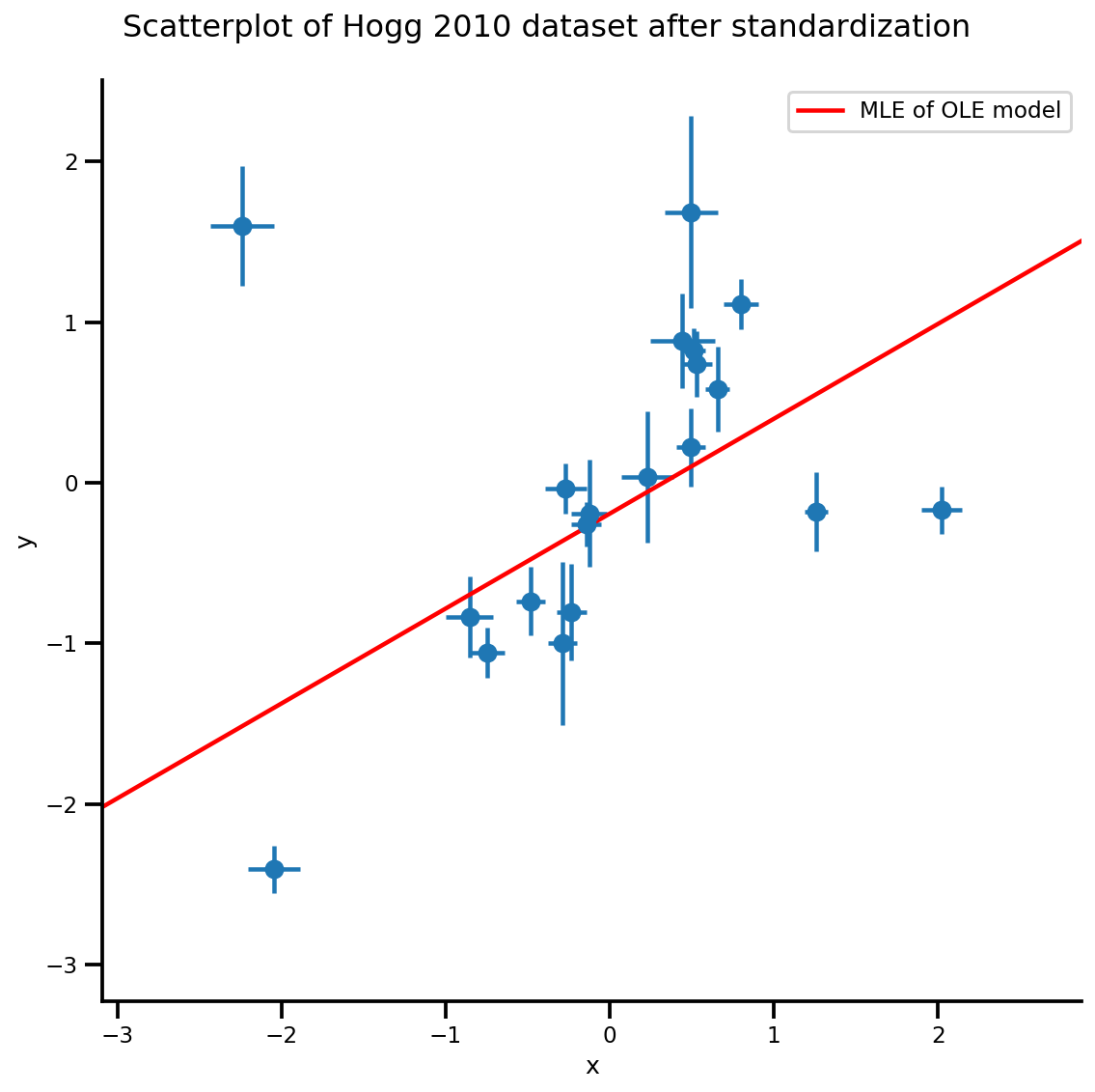
b0est, b1est = lbfgs_results.position.numpy()

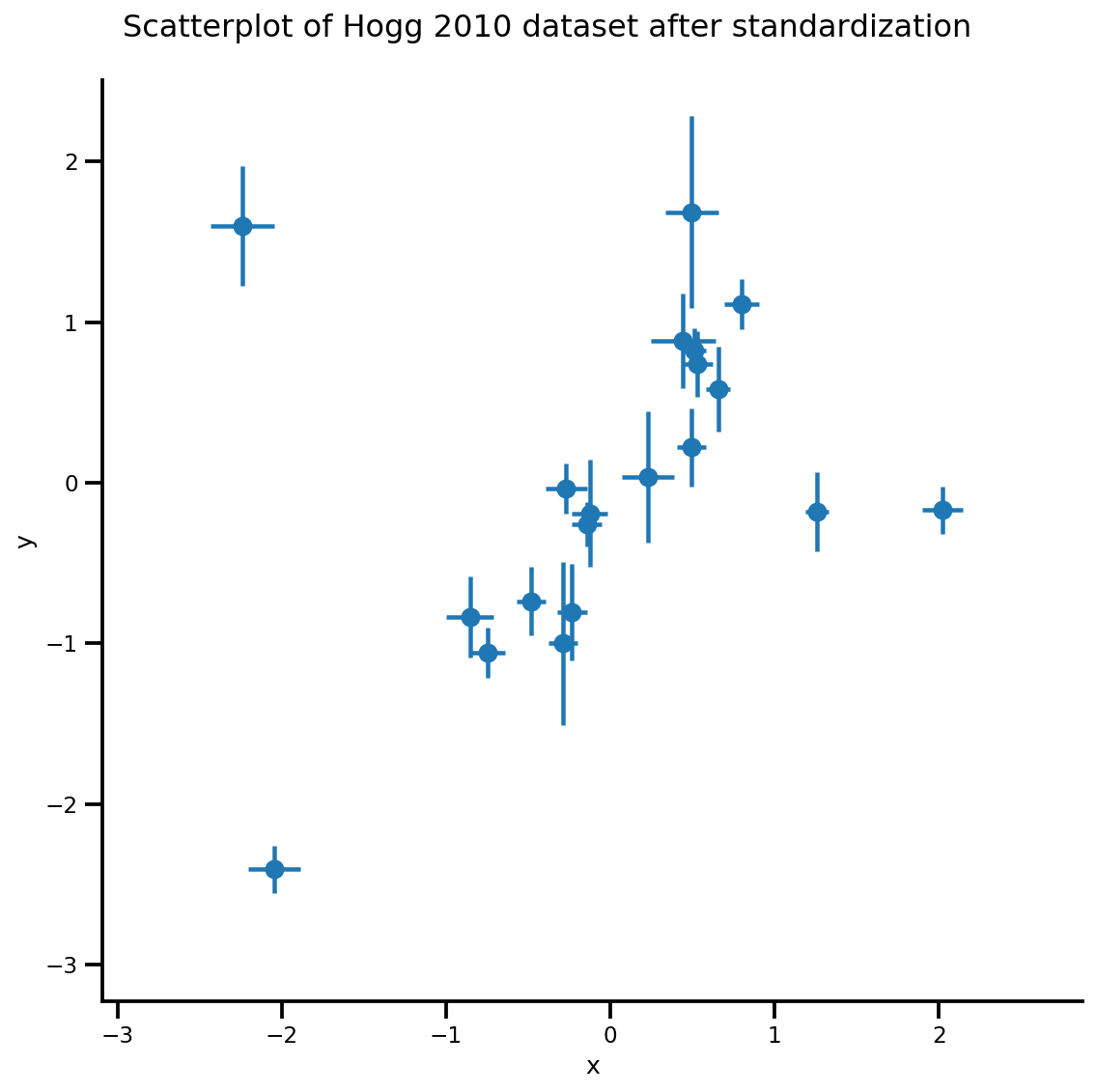
g, xlims, ylims = plot_hoggs(dfhoggs);
xrange = np.linspace(xlims[0], xlims[1], 100)
g.axes[0][0].plot(xrange, b0est + b1est*xrange, 
                  color='r', label='MLE of OLE model')
plt.legend();

/usr/local/lib/python3.6/dist-packages/numpy/core/fromnumeric.py:2495: FutureWarning: Method .ptp is deprecated and will be removed in a future version. Use numpy.ptp instead.
  return ptp(axis=axis, out=out, **kwargs)
/usr/local/lib/python3.6/dist-packages/seaborn/axisgrid.py:230: UserWarning: The `size` paramter has been renamed to `height`; please update your code.
  warnings.warn(msg, UserWarning)

批次版本模型和 MCMC

在貝氏推論中，我們通常希望使用 MCMC 樣本，因為當樣本來自後驗時，我們可以將它們插入任何函數中來計算期望值。但是，MCMC API 要求我們編寫批次友善的模型，我們可以透過呼叫 sample([...]) 來檢查我們的模型實際上是否「可批次化」

mdl_ols_.sample(5)  # <== error as some computation could not be broadcasted.

在這種情況下，這相對簡單，因為我們的模型內部只有一個線性函數，擴展形狀應該就能解決問題

mdl_ols_batch = tfd.JointDistributionSequential([
    # b0
    tfd.Normal(loc=tf.cast(0, dtype), scale=1.),
    # b1
    tfd.Normal(loc=tf.cast(0, dtype), scale=1.),
    # likelihood
    #   Using Independent to ensure the log_prob is not incorrectly broadcasted
    lambda b1, b0: tfd.Independent(
        tfd.Normal(
            # Parameter transformation
            loc=b0[..., tf.newaxis] + b1[..., tf.newaxis]*X_np[tf.newaxis, ...],
            scale=sigma_y_np[tf.newaxis, ...]),
        reinterpreted_batch_ndims=1
    ),
])

mdl_ols_batch.resolve_graph()

(('b0', ()), ('b1', ()), ('x', ('b1', 'b0')))

我們可以再次抽樣並評估 log_prob_parts 以進行一些檢查

b0, b1, y = mdl_ols_batch.sample(4)
mdl_ols_batch.log_prob_parts([b0, b1, y])

[<tf.Tensor: shape=(4,), dtype=float64, numpy=array([-1.25230168, -1.45281432, -1.87110061, -1.07665206])>,
 <tf.Tensor: shape=(4,), dtype=float64, numpy=array([-1.07019936, -1.59562117, -2.53387765, -1.01557632])>,
 <tf.Tensor: shape=(4,), dtype=float64, numpy=array([ 0.45841406,  2.56829635, -4.84973951, -5.59423992])>]

一些附註

• 我們希望使用模型的批次版本，因為它對於多鏈 MCMC 來說速度最快。如果您無法將模型重寫為批次版本（例如，ODE 模型），您可以使用 tf.map_fn 對 log_prob 函數進行映射，以達到相同的效果。
• 現在 mdl_ols_batch.sample() 可能無法運作，因為我們有純量先驗，因為我們無法執行 scaler_tensor[:, None]。此處的解決方案是透過包裝 tfd.Sample(..., sample_shape=1) 將純量張量擴展為等級 1。
• 最好將模型寫成函數，這樣您就可以更輕鬆地變更超參數等設定。

def gen_ols_batch_model(X, sigma, hyperprior_mean=0, hyperprior_scale=1):
  hyper_mean = tf.cast(hyperprior_mean, dtype)
  hyper_scale = tf.cast(hyperprior_scale, dtype)
  return tfd.JointDistributionSequential([
      # b0
      tfd.Sample(tfd.Normal(loc=hyper_mean, scale=hyper_scale), sample_shape=1),
      # b1
      tfd.Sample(tfd.Normal(loc=hyper_mean, scale=hyper_scale), sample_shape=1),
      # likelihood
      lambda b1, b0: tfd.Independent(
          tfd.Normal(
              # Parameter transformation
              loc=b0 + b1*X,
              scale=sigma),
          reinterpreted_batch_ndims=1
      ),
  ], validate_args=True)

mdl_ols_batch = gen_ols_batch_model(X_np[tf.newaxis, ...],
                                    sigma_y_np[tf.newaxis, ...])

_ = mdl_ols_batch.sample()
_ = mdl_ols_batch.sample(4)
_ = mdl_ols_batch.sample([3, 4])

# Small helper function to validate log_prob shape (avoid wrong broadcasting)
def validate_log_prob_part(model, batch_shape=1, observed=-1):
  samples = model.sample(batch_shape)
  logp_part = list(model.log_prob_parts(samples))

  # exclude observed node
  logp_part.pop(observed)
  for part in logp_part:
    tf.assert_equal(part.shape, logp_part[-1].shape)

validate_log_prob_part(mdl_ols_batch, 4)

更多檢查：比較產生的 log_prob 函數與手寫的 TFP log_prob 函數。

def ols_logp_batch(b0, b1, Y):
  b0_prior = tfd.Normal(loc=tf.cast(0, dtype), scale=1.) # b0
  b1_prior = tfd.Normal(loc=tf.cast(0, dtype), scale=1.) # b1
  likelihood = tfd.Normal(loc=b0 + b1*X_np[None, :],
                          scale=sigma_y_np) # likelihood
  return tf.reduce_sum(b0_prior.log_prob(b0), axis=-1) +\
         tf.reduce_sum(b1_prior.log_prob(b1), axis=-1) +\
         tf.reduce_sum(likelihood.log_prob(Y), axis=-1)

b0, b1, x = mdl_ols_batch.sample(4)
print(mdl_ols_batch.log_prob([b0, b1, Y_np]).numpy()) 
print(ols_logp_batch(b0, b1, Y_np).numpy())

[-227.37899384 -327.10043743 -570.44162789 -702.79808683]
[-227.37899384 -327.10043743 -570.44162789 -702.79808683]

使用 No-U-Turn Sampler 的 MCMC

常見的 run_chain 函數

@tf.function(autograph=False, experimental_compile=True)
def run_chain(init_state, step_size, target_log_prob_fn, unconstraining_bijectors,
              num_steps=500, burnin=50):

  def trace_fn(_, pkr):
    return (
        pkr.inner_results.inner_results.target_log_prob,
        pkr.inner_results.inner_results.leapfrogs_taken,
        pkr.inner_results.inner_results.has_divergence,
        pkr.inner_results.inner_results.energy,
        pkr.inner_results.inner_results.log_accept_ratio
           )

  kernel = tfp.mcmc.TransformedTransitionKernel(
    inner_kernel=tfp.mcmc.NoUTurnSampler(
      target_log_prob_fn,
      step_size=step_size),
    bijector=unconstraining_bijectors)

  hmc = tfp.mcmc.DualAveragingStepSizeAdaptation(
    inner_kernel=kernel,
    num_adaptation_steps=burnin,
    step_size_setter_fn=lambda pkr, new_step_size: pkr._replace(
        inner_results=pkr.inner_results._replace(step_size=new_step_size)),
    step_size_getter_fn=lambda pkr: pkr.inner_results.step_size,
    log_accept_prob_getter_fn=lambda pkr: pkr.inner_results.log_accept_ratio
  )

  # Sampling from the chain.
  chain_state, sampler_stat = tfp.mcmc.sample_chain(
      num_results=num_steps,
      num_burnin_steps=burnin,
      current_state=init_state,
      kernel=hmc,
      trace_fn=trace_fn)
  return chain_state, sampler_stat

nchain = 10
b0, b1, _ = mdl_ols_batch.sample(nchain)
init_state = [b0, b1]
step_size = [tf.cast(i, dtype=dtype) for i in [.1, .1]]
target_log_prob_fn = lambda *x: mdl_ols_batch.log_prob(x + (Y_np, ))

# bijector to map contrained parameters to real
unconstraining_bijectors = [
    tfb.Identity(),
    tfb.Identity(),
]

samples, sampler_stat = run_chain(
    init_state, step_size, target_log_prob_fn, unconstraining_bijectors)

# using the pymc3 naming convention
sample_stats_name = ['lp', 'tree_size', 'diverging', 'energy', 'mean_tree_accept']
sample_stats = {k:v.numpy().T for k, v in zip(sample_stats_name, sampler_stat)}
sample_stats['tree_size'] = np.diff(sample_stats['tree_size'], axis=1)

var_name = ['b0', 'b1']
posterior = {k:np.swapaxes(v.numpy(), 1, 0) 
             for k, v in zip(var_name, samples)}

az_trace = az.from_dict(posterior=posterior, sample_stats=sample_stats)

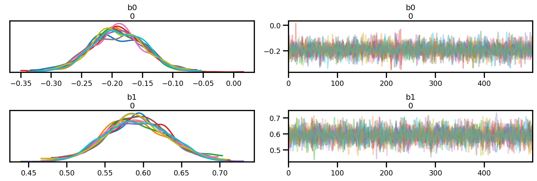
az.plot_trace(az_trace);

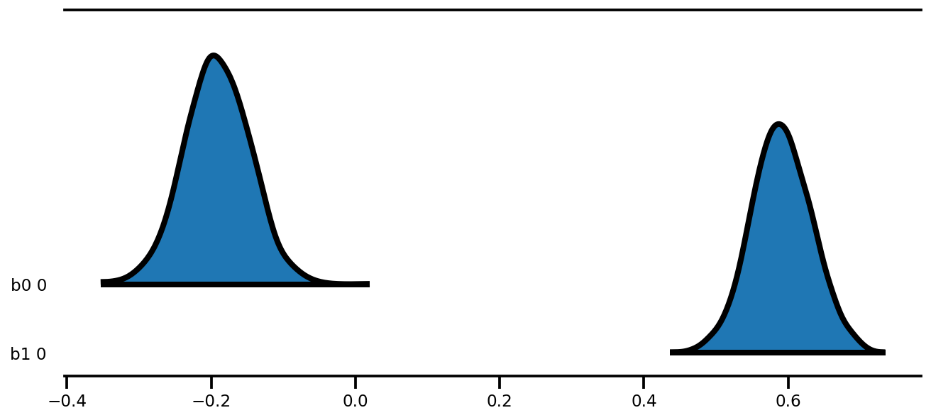
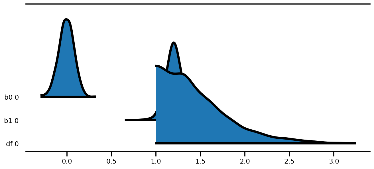
az.plot_forest(az_trace,
               kind='ridgeplot',
               linewidth=4,
               combined=True,
               ridgeplot_overlap=1.5,
               figsize=(9, 4));

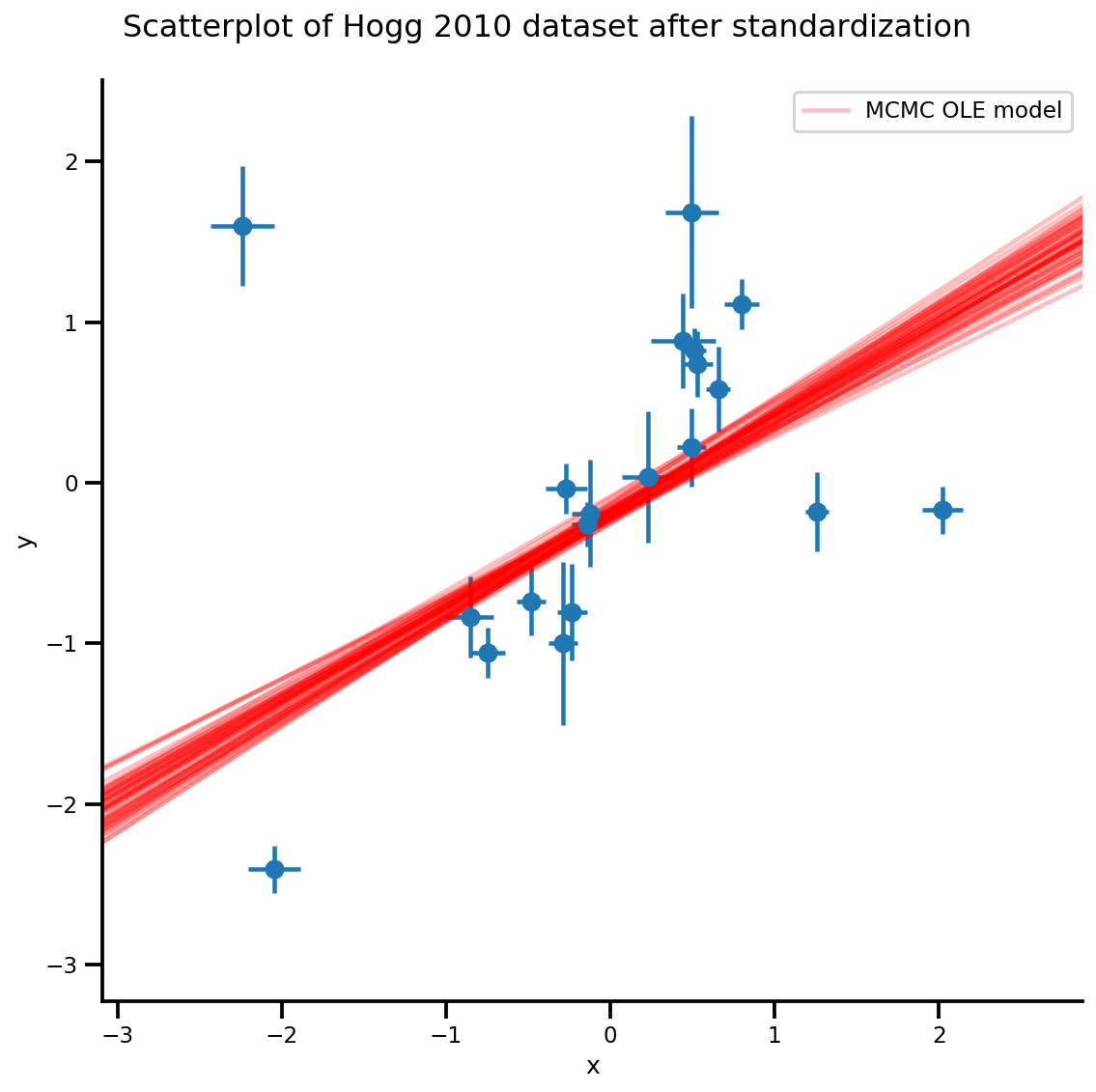
k = 5
b0est, b1est = az_trace.posterior['b0'][:, -k:].values, az_trace.posterior['b1'][:, -k:].values

g, xlims, ylims = plot_hoggs(dfhoggs);
xrange = np.linspace(xlims[0], xlims[1], 100)[None, :]
g.axes[0][0].plot(np.tile(xrange, (k, 1)).T,
                  (np.reshape(b0est, [-1, 1]) + np.reshape(b1est, [-1, 1])*xrange).T,
                  alpha=.25, color='r')
plt.legend([g.axes[0][0].lines[-1]], ['MCMC OLE model']);

/usr/local/lib/python3.6/dist-packages/numpy/core/fromnumeric.py:2495: FutureWarning: Method .ptp is deprecated and will be removed in a future version. Use numpy.ptp instead.
  return ptp(axis=axis, out=out, **kwargs)
/usr/local/lib/python3.6/dist-packages/seaborn/axisgrid.py:230: UserWarning: The `size` paramter has been renamed to `height`; please update your code.
  warnings.warn(msg, UserWarning)
/usr/local/lib/python3.6/dist-packages/ipykernel_launcher.py:8: MatplotlibDeprecationWarning: cycling among columns of inputs with non-matching shapes is deprecated.

Student-T 方法

請注意，從現在開始我們一律使用模型的批次版本

def gen_studentt_model(X, sigma,
                       hyper_mean=0, hyper_scale=1, lower=1, upper=100):
  loc = tf.cast(hyper_mean, dtype)
  scale = tf.cast(hyper_scale, dtype)
  low = tf.cast(lower, dtype)
  high = tf.cast(upper, dtype)
  return tfd.JointDistributionSequential([
      # b0 ~ Normal(0, 1)
      tfd.Sample(tfd.Normal(loc, scale), sample_shape=1),
      # b1 ~ Normal(0, 1)
      tfd.Sample(tfd.Normal(loc, scale), sample_shape=1),
      # df ~ Uniform(a, b)
      tfd.Sample(tfd.Uniform(low, high), sample_shape=1),
      # likelihood ~ StudentT(df, f(b0, b1), sigma_y)
      #   Using Independent to ensure the log_prob is not incorrectly broadcasted.
      lambda df, b1, b0: tfd.Independent(
          tfd.StudentT(df=df, loc=b0 + b1*X, scale=sigma)),
  ], validate_args=True)

mdl_studentt = gen_studentt_model(X_np[tf.newaxis, ...],
                                  sigma_y_np[tf.newaxis, ...])
mdl_studentt.resolve_graph()

(('b0', ()), ('b1', ()), ('df', ()), ('x', ('df', 'b1', 'b0')))

validate_log_prob_part(mdl_studentt, 4)

前向抽樣（先驗預測抽樣）

b0, b1, df, x = mdl_studentt.sample(1000)
x.shape

TensorShape([1000, 20])

MLE

# bijector to map contrained parameters to real
a, b = tf.constant(1., dtype), tf.constant(100., dtype),

# Interval transformation
tfp_interval = tfb.Inline(
    inverse_fn=(
        lambda x: tf.math.log(x - a) - tf.math.log(b - x)),
    forward_fn=(
        lambda y: (b - a) * tf.sigmoid(y) + a),
    forward_log_det_jacobian_fn=(
        lambda x: tf.math.log(b - a) - 2 * tf.nn.softplus(-x) - x),
    forward_min_event_ndims=0,
    name="interval")

unconstraining_bijectors = [
    tfb.Identity(),
    tfb.Identity(),
    tfp_interval,
]

mapper = Mapper(mdl_studentt.sample()[:-1],
                unconstraining_bijectors,
                mdl_studentt.event_shape[:-1])

@_make_val_and_grad_fn
def neg_log_likelihood(x):
  # Generate a function closure so that we are computing the log_prob
  # conditioned on the observed data. Note also that tfp.optimizer.* takes a 
  # single tensor as input, so we need to do some slicing here:
  return -tf.squeeze(mdl_studentt.log_prob(
      mapper.split_and_reshape(x) + [Y_np]))

lbfgs_results = tfp.optimizer.lbfgs_minimize(
    neg_log_likelihood,
    initial_position=mapper.flatten_and_concat(mdl_studentt.sample()[:-1]),
    tolerance=1e-20,
    x_tolerance=1e-20
)

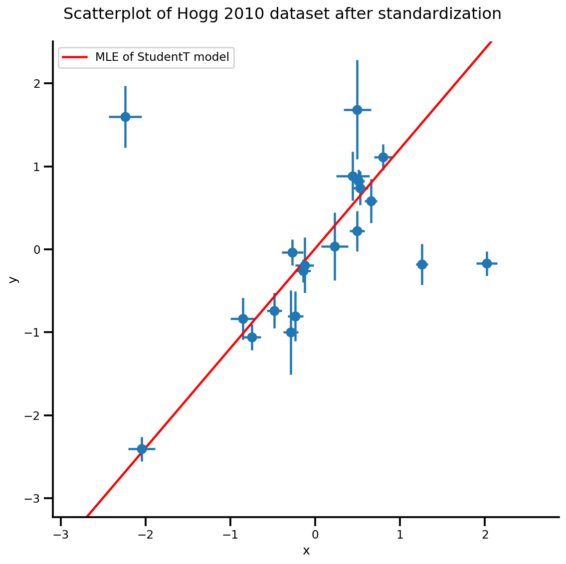
b0est, b1est, dfest = lbfgs_results.position.numpy()

g, xlims, ylims = plot_hoggs(dfhoggs);
xrange = np.linspace(xlims[0], xlims[1], 100)
g.axes[0][0].plot(xrange, b0est + b1est*xrange, 
                  color='r', label='MLE of StudentT model')
plt.legend();

/usr/local/lib/python3.6/dist-packages/numpy/core/fromnumeric.py:2495: FutureWarning: Method .ptp is deprecated and will be removed in a future version. Use numpy.ptp instead.
  return ptp(axis=axis, out=out, **kwargs)
/usr/local/lib/python3.6/dist-packages/seaborn/axisgrid.py:230: UserWarning: The `size` paramter has been renamed to `height`; please update your code.
  warnings.warn(msg, UserWarning)

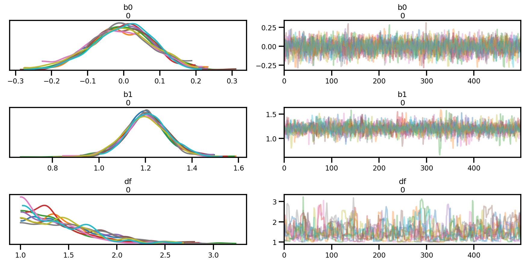
MCMC

nchain = 10
b0, b1, df, _ = mdl_studentt.sample(nchain)
init_state = [b0, b1, df]
step_size = [tf.cast(i, dtype=dtype) for i in [.1, .1, .05]]

target_log_prob_fn = lambda *x: mdl_studentt.log_prob(x + (Y_np, ))

samples, sampler_stat = run_chain(
    init_state, step_size, target_log_prob_fn, unconstraining_bijectors, burnin=100)

# using the pymc3 naming convention
sample_stats_name = ['lp', 'tree_size', 'diverging', 'energy', 'mean_tree_accept']
sample_stats = {k:v.numpy().T for k, v in zip(sample_stats_name, sampler_stat)}
sample_stats['tree_size'] = np.diff(sample_stats['tree_size'], axis=1)

var_name = ['b0', 'b1', 'df']
posterior = {k:np.swapaxes(v.numpy(), 1, 0) 
             for k, v in zip(var_name, samples)}

az_trace = az.from_dict(posterior=posterior, sample_stats=sample_stats)

az.summary(az_trace)

az.plot_trace(az_trace);

az.plot_forest(az_trace,
               kind='ridgeplot',
               linewidth=4,
               combined=True,
               ridgeplot_overlap=1.5,
               figsize=(9, 4));

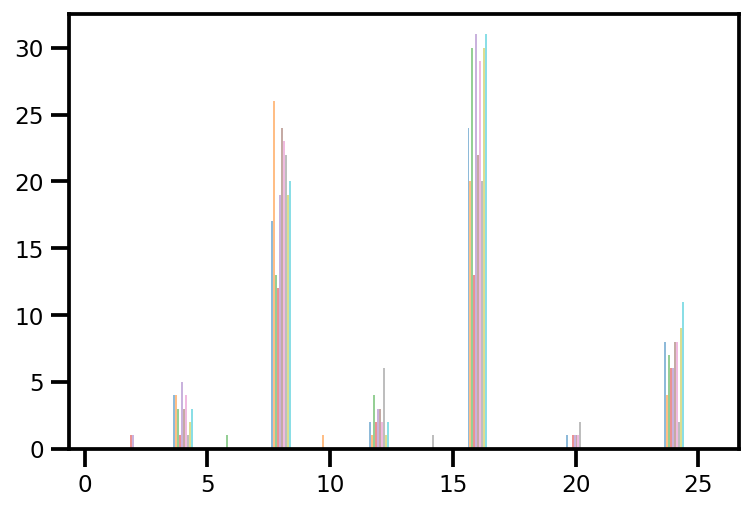
plt.hist(az_trace.sample_stats['tree_size'], np.linspace(.5, 25.5, 26), alpha=.5);

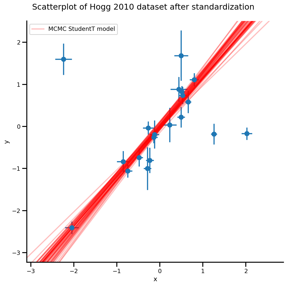
k = 5
b0est, b1est = az_trace.posterior['b0'][:, -k:].values, az_trace.posterior['b1'][:, -k:].values

g, xlims, ylims = plot_hoggs(dfhoggs);
xrange = np.linspace(xlims[0], xlims[1], 100)[None, :]
g.axes[0][0].plot(np.tile(xrange, (k, 1)).T,
                  (np.reshape(b0est, [-1, 1]) + np.reshape(b1est, [-1, 1])*xrange).T,
                  alpha=.25, color='r')
plt.legend([g.axes[0][0].lines[-1]], ['MCMC StudentT model']);

/usr/local/lib/python3.6/dist-packages/numpy/core/fromnumeric.py:2495: FutureWarning: Method .ptp is deprecated and will be removed in a future version. Use numpy.ptp instead.
  return ptp(axis=axis, out=out, **kwargs)
/usr/local/lib/python3.6/dist-packages/seaborn/axisgrid.py:230: UserWarning: The `size` paramter has been renamed to `height`; please update your code.
  warnings.warn(msg, UserWarning)
/usr/local/lib/python3.6/dist-packages/ipykernel_launcher.py:8: MatplotlibDeprecationWarning: cycling among columns of inputs with non-matching shapes is deprecated.

階層式部分共用

出自 PyMC3 Efron 和 Morris (1975) 針對 18 位球員的棒球數據

data = pd.read_table('https://raw.githubusercontent.com/pymc-devs/pymc3/master/pymc3/examples/data/efron-morris-75-data.tsv',
                     sep="\t")
at_bats, hits = data[['At-Bats', 'Hits']].values.T
n = len(at_bats)

def gen_baseball_model(at_bats, rate=1.5, a=0, b=1):
  return tfd.JointDistributionSequential([
    # phi
    tfd.Uniform(low=tf.cast(a, dtype), high=tf.cast(b, dtype)),
    # kappa_log
    tfd.Exponential(rate=tf.cast(rate, dtype)),
    # thetas
    lambda kappa_log, phi: tfd.Sample(
        tfd.Beta(
            concentration1=tf.exp(kappa_log)*phi,
            concentration0=tf.exp(kappa_log)*(1.0-phi)),
        sample_shape=n
    ),
    # likelihood
    lambda thetas: tfd.Independent(
        tfd.Binomial(
            total_count=tf.cast(at_bats, dtype),
            probs=thetas
        )), 
])

mdl_baseball = gen_baseball_model(at_bats)
mdl_baseball.resolve_graph()

(('phi', ()),
 ('kappa_log', ()),
 ('thetas', ('kappa_log', 'phi')),
 ('x', ('thetas',)))

前向抽樣（先驗預測抽樣）

phi, kappa_log, thetas, y = mdl_baseball.sample(4)
# phi, kappa_log, thetas, y

再次提醒，請注意如果您不使用 Independent，最終會得到具有錯誤 batch_shape 的 log_prob。

# check logp
pprint(mdl_baseball.log_prob_parts([phi, kappa_log, thetas, hits]))
print(mdl_baseball.log_prob([phi, kappa_log, thetas, hits]))

[<tf.Tensor: shape=(4,), dtype=float64, numpy=array([0., 0., 0., 0.])>,
 <tf.Tensor: shape=(4,), dtype=float64, numpy=array([ 0.1721297 , -0.95946498, -0.72591188,  0.23993813])>,
 <tf.Tensor: shape=(4,), dtype=float64, numpy=array([59.35192283,  7.0650634 ,  0.83744911, 74.14370935])>,
 <tf.Tensor: shape=(4,), dtype=float64, numpy=array([-3279.75191016,  -931.10438484,  -512.59197688, -1131.08043597])>]
tf.Tensor([-3220.22785762  -924.99878641  -512.48043966 -1056.69678849], shape=(4,), dtype=float64)

MLE

tfp.optimizer 一個非常棒的功能是，您可以針對 k 個起點批次平行最佳化，並指定 stopping_condition kwarg：您可以將其設定為 tfp.optimizer.converged_all，以查看它們是否都找到相同的最小值，或設定為 tfp.optimizer.converged_any 以快速找到局部解。

unconstraining_bijectors = [
    tfb.Sigmoid(),
    tfb.Exp(),
    tfb.Sigmoid(),
]

phi, kappa_log, thetas, y = mdl_baseball.sample(10)

mapper = Mapper([phi, kappa_log, thetas],
                unconstraining_bijectors,
                mdl_baseball.event_shape[:-1])

@_make_val_and_grad_fn
def neg_log_likelihood(x):
  return -mdl_baseball.log_prob(mapper.split_and_reshape(x) + [hits])

start = mapper.flatten_and_concat([phi, kappa_log, thetas])

lbfgs_results = tfp.optimizer.lbfgs_minimize(
    neg_log_likelihood,
    num_correction_pairs=10,
    initial_position=start,
    # lbfgs actually can work in batch as well
    stopping_condition=tfp.optimizer.converged_any,
    tolerance=1e-50,
    x_tolerance=1e-50,
    parallel_iterations=10,
    max_iterations=200
)

lbfgs_results.converged.numpy(), lbfgs_results.failed.numpy()

(array([False, False, False, False, False, False, False, False, False,
        False]),
 array([ True,  True,  True,  True,  True,  True,  True,  True,  True,
         True]))

result = lbfgs_results.position[lbfgs_results.converged & ~lbfgs_results.failed]
result

<tf.Tensor: shape=(0, 20), dtype=float64, numpy=array([], shape=(0, 20), dtype=float64)>

LBFGS 未收斂。

if result.shape[0] > 0:
  phi_est, kappa_est, theta_est = mapper.split_and_reshape(result)
  phi_est, kappa_est, theta_est

MCMC

target_log_prob_fn = lambda *x: mdl_baseball.log_prob(x + (hits, ))

nchain = 4
phi, kappa_log, thetas, _ = mdl_baseball.sample(nchain)
init_state = [phi, kappa_log, thetas]
step_size=[tf.cast(i, dtype=dtype) for i in [.1, .1, .1]]

samples, sampler_stat = run_chain(
    init_state, step_size, target_log_prob_fn, unconstraining_bijectors,
    burnin=200)

# using the pymc3 naming convention
sample_stats_name = ['lp', 'tree_size', 'diverging', 'energy', 'mean_tree_accept']
sample_stats = {k:v.numpy().T for k, v in zip(sample_stats_name, sampler_stat)}
sample_stats['tree_size'] = np.diff(sample_stats['tree_size'], axis=1)

var_name = ['phi', 'kappa_log', 'thetas']
posterior = {k:np.swapaxes(v.numpy(), 1, 0) 
             for k, v in zip(var_name, samples)}

az_trace = az.from_dict(posterior=posterior, sample_stats=sample_stats)

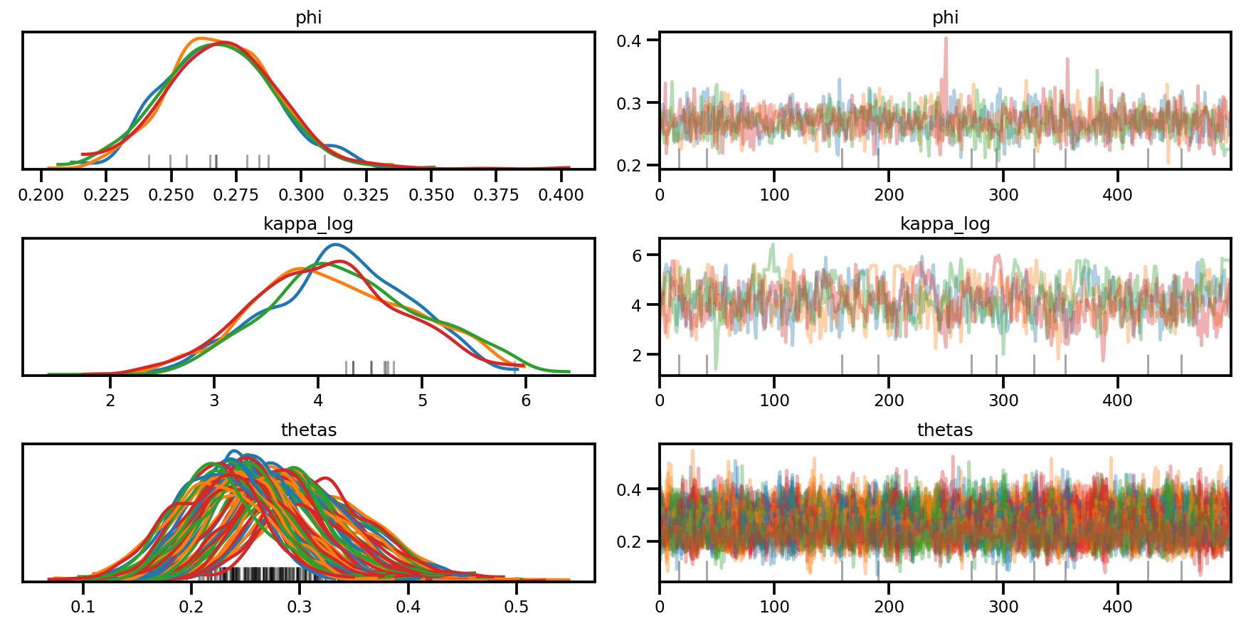
az.plot_trace(az_trace, compact=True);

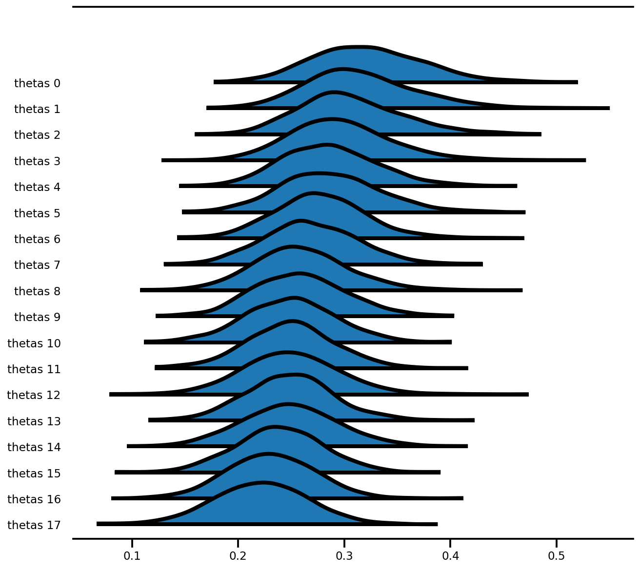
az.plot_forest(az_trace,
               var_names=['thetas'],
               kind='ridgeplot',
               linewidth=4,
               combined=True,
               ridgeplot_overlap=1.5,
               figsize=(9, 8));

混合效應模型 (氡)

PyMC3 文件中的最後一個模型：多層次建模的貝氏方法入門

先驗的一些變更（較小規模等等）

載入原始資料並清理

srrs2 = pd.read_csv('https://raw.githubusercontent.com/pymc-devs/pymc3/master/pymc3/examples/data/srrs2.dat')

srrs2.columns = srrs2.columns.map(str.strip)
srrs_mn = srrs2[srrs2.state=='MN'].copy()
srrs_mn['fips'] = srrs_mn.stfips*1000 + srrs_mn.cntyfips

cty = pd.read_csv('https://raw.githubusercontent.com/pymc-devs/pymc3/master/pymc3/examples/data/cty.dat')
cty_mn = cty[cty.st=='MN'].copy()
cty_mn[ 'fips'] = 1000*cty_mn.stfips + cty_mn.ctfips

srrs_mn = srrs_mn.merge(cty_mn[['fips', 'Uppm']], on='fips')
srrs_mn = srrs_mn.drop_duplicates(subset='idnum')
u = np.log(srrs_mn.Uppm)

n = len(srrs_mn)

srrs_mn.county = srrs_mn.county.map(str.strip)
mn_counties = srrs_mn.county.unique()
counties = len(mn_counties)
county_lookup = dict(zip(mn_counties, range(len(mn_counties))))

county = srrs_mn['county_code'] = srrs_mn.county.replace(county_lookup).values
radon = srrs_mn.activity
srrs_mn['log_radon'] = log_radon = np.log(radon + 0.1).values
floor_measure = srrs_mn.floor.values.astype('float')

# Create new variable for mean of floor across counties
xbar = srrs_mn.groupby('county')['floor'].mean().rename(county_lookup).values

對於具有複雜轉換的模型，以函數式風格實作會讓編寫和測試更加容易。此外，它也讓以程式設計方式產生以（小批次）輸入資料為條件的 log_prob 函數變得更加容易

def affine(u_val, x_county, county, floor, gamma, eps, b):
  """Linear equation of the coefficients and the covariates, with broadcasting."""
  return (tf.transpose((gamma[..., 0]
                      + gamma[..., 1]*u_val[:, None]
                      + gamma[..., 2]*x_county[:, None]))
          + tf.gather(eps, county, axis=-1)
          + b*floor)


def gen_radon_model(u_val, x_county, county, floor,
                    mu0=tf.zeros([], dtype, name='mu0')):
  """Creates a joint distribution representing our generative process."""
  return tfd.JointDistributionSequential([
      # sigma_a
      tfd.HalfCauchy(loc=mu0, scale=5.),
      # eps
      lambda sigma_a: tfd.Sample(
          tfd.Normal(loc=mu0, scale=sigma_a), sample_shape=counties),
      # gamma
      tfd.Sample(tfd.Normal(loc=mu0, scale=100.), sample_shape=3),
      # b
      tfd.Sample(tfd.Normal(loc=mu0, scale=100.), sample_shape=1),
      # sigma_y
      tfd.Sample(tfd.HalfCauchy(loc=mu0, scale=5.), sample_shape=1),
      # likelihood
      lambda sigma_y, b, gamma, eps: tfd.Independent(
          tfd.Normal(
              loc=affine(u_val, x_county, county, floor, gamma, eps, b),
              scale=sigma_y
          ),
          reinterpreted_batch_ndims=1
      ),
  ])

contextual_effect2 = gen_radon_model(
    u.values,  xbar[county], county, floor_measure)

@tf.function(autograph=False)
def unnormalized_posterior_log_prob(sigma_a, gamma, eps, b, sigma_y):
  """Computes `joint_log_prob` pinned at `log_radon`."""
  return contextual_effect2.log_prob(
      [sigma_a, gamma, eps, b, sigma_y, log_radon])

assert [4] == unnormalized_posterior_log_prob(
    *contextual_effect2.sample(4)[:-1]).shape

samples = contextual_effect2.sample(4)
pprint([s.shape for s in samples])

[TensorShape([4]),
 TensorShape([4, 85]),
 TensorShape([4, 3]),
 TensorShape([4, 1]),
 TensorShape([4, 1]),
 TensorShape([4, 919])]

contextual_effect2.log_prob_parts(list(samples)[:-1] + [log_radon])

[<tf.Tensor: shape=(4,), dtype=float64, numpy=array([-3.95681828, -2.45693443, -2.53310078, -4.7717536 ])>,
 <tf.Tensor: shape=(4,), dtype=float64, numpy=array([-340.65975204, -217.11139018, -246.50498667, -369.79687704])>,
 <tf.Tensor: shape=(4,), dtype=float64, numpy=array([-20.49822449, -20.38052557, -18.63843525, -17.83096972])>,
 <tf.Tensor: shape=(4,), dtype=float64, numpy=array([-5.94765605, -5.91460848, -6.66169402, -5.53894593])>,
 <tf.Tensor: shape=(4,), dtype=float64, numpy=array([-2.10293999, -4.34186631, -2.10744955, -3.016717  ])>,
 <tf.Tensor: shape=(4,), dtype=float64, numpy=
 array([-29022322.1413861 ,   -114422.36893361,  -8708500.81752865,
           -35061.92497235])>]

變分推論

JointDistribution* 一個非常強大的功能是，您可以輕鬆地為 VI 產生近似值。例如，若要執行平均場 ADVI，您只需檢查圖形，並將所有未觀察到的分佈替換為常態分佈。

平均場 ADVI

您也可以使用 tensorflow_probability/python/experimental/vi 中的實驗性功能來建構變分近似值，這些近似值基本上與下面使用的邏輯相同（即使用 JointDistribution 建構近似值），但近似值輸出在原始空間中，而不是在無界空間中。

from tensorflow_probability.python.mcmc.transformed_kernel import (
    make_transform_fn, make_transformed_log_prob)

# Wrap logp so that all parameters are in the Real domain
# copied and edited from tensorflow_probability/python/mcmc/transformed_kernel.py
unconstraining_bijectors = [
    tfb.Exp(),
    tfb.Identity(),
    tfb.Identity(),
    tfb.Identity(),
    tfb.Exp()
]

unnormalized_log_prob = lambda *x: contextual_effect2.log_prob(x + (log_radon,))

contextual_effect_posterior = make_transformed_log_prob(
    unnormalized_log_prob,
    unconstraining_bijectors,
    direction='forward',
    # TODO(b/72831017): Disable caching until gradient linkage
    # generally works.
    enable_bijector_caching=False)

# debug
if True:
  # Check the two versions of log_prob - they should be different given the Jacobian
  rv_samples = contextual_effect2.sample(4)

  _inverse_transform = make_transform_fn(unconstraining_bijectors, 'inverse')
  _forward_transform = make_transform_fn(unconstraining_bijectors, 'forward')

  pprint([
      unnormalized_log_prob(*rv_samples[:-1]),
      contextual_effect_posterior(*_inverse_transform(rv_samples[:-1])),
      unnormalized_log_prob(
          *_forward_transform(
              tf.zeros_like(a, dtype=dtype) for a in rv_samples[:-1])
      ),
      contextual_effect_posterior(
          *[tf.zeros_like(a, dtype=dtype) for a in rv_samples[:-1]]
      ),
  ])

[<tf.Tensor: shape=(4,), dtype=float64, numpy=array([-1.73354969e+04, -5.51622488e+04, -2.77754609e+08, -1.09065161e+07])>,
 <tf.Tensor: shape=(4,), dtype=float64, numpy=array([-1.73331358e+04, -5.51582029e+04, -2.77754602e+08, -1.09065134e+07])>,
 <tf.Tensor: shape=(4,), dtype=float64, numpy=array([-1992.10420767, -1992.10420767, -1992.10420767, -1992.10420767])>,
 <tf.Tensor: shape=(4,), dtype=float64, numpy=array([-1992.10420767, -1992.10420767, -1992.10420767, -1992.10420767])>]

# Build meanfield ADVI for a jointdistribution
# Inspect the input jointdistribution and replace the list of distribution with
# a list of Normal distribution, each with the same shape.
def build_meanfield_advi(jd_list, observed_node=-1):
  """
  The inputted jointdistribution needs to be a batch version
  """
  # Sample to get a list of Tensors
  list_of_values = jd_list.sample(1)  # <== sample([]) might not work

  # Remove the observed node
  list_of_values.pop(observed_node)

  # Iterate the list of Tensor to a build a list of Normal distribution (i.e.,
  # the Variational posterior)
  distlist = []
  for i, value in enumerate(list_of_values):
    dtype = value.dtype
    rv_shape = value[0].shape
    loc = tf.Variable(
        tf.random.normal(rv_shape, dtype=dtype),
        name='meanfield_%s_mu' % i,
        dtype=dtype)
    scale = tfp.util.TransformedVariable(
        tf.fill(rv_shape, value=tf.constant(0.02, dtype)),
        tfb.Softplus(),
        name='meanfield_%s_scale' % i,
    )

    approx_node = tfd.Normal(loc=loc, scale=scale)
    if loc.shape == ():
      distlist.append(approx_node)
    else:
      distlist.append(
          # TODO: make the reinterpreted_batch_ndims more flexible (for 
          # minibatch etc)
          tfd.Independent(approx_node, reinterpreted_batch_ndims=1)
      )

  # pass list to JointDistribution to initiate the meanfield advi
  meanfield_advi = tfd.JointDistributionSequential(distlist)
  return meanfield_advi

advi = build_meanfield_advi(contextual_effect2, observed_node=-1)

# Check the logp and logq
advi_samples = advi.sample(4)
pprint([
  advi.log_prob(advi_samples),
  contextual_effect_posterior(*advi_samples)
  ])

[<tf.Tensor: shape=(4,), dtype=float64, numpy=array([231.26836839, 229.40755095, 227.10287879, 224.05914594])>,
 <tf.Tensor: shape=(4,), dtype=float64, numpy=array([-10615.93542431, -11743.21420129, -10376.26732337, -11338.00600103])>]

opt = tf_keras.optimizers.Adam(learning_rate=.1)

@tf.function(experimental_compile=True)
def run_approximation():
  loss_ = tfp.vi.fit_surrogate_posterior(
        contextual_effect_posterior,
        surrogate_posterior=advi,
        optimizer=opt,
        sample_size=10,
        num_steps=300)
  return loss_

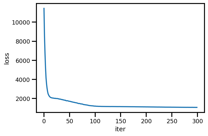
loss_ = run_approximation()

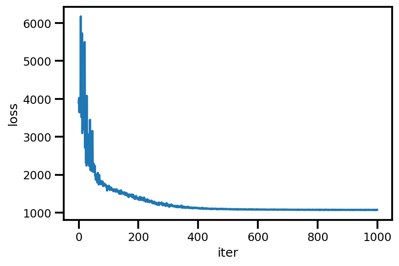
plt.plot(loss_);
plt.xlabel('iter');
plt.ylabel('loss');

graph_info = contextual_effect2.resolve_graph()
approx_param = dict()
free_param = advi.trainable_variables
for i, (rvname, param) in enumerate(graph_info[:-1]):
  approx_param[rvname] = {"mu": free_param[i*2].numpy(),
                          "sd": free_param[i*2+1].numpy()}

approx_param.keys()

dict_keys(['sigma_a', 'eps', 'gamma', 'b', 'sigma_y'])

approx_param['gamma']

{'mu': array([1.28145814, 0.70365287, 1.02689857]),
 'sd': array([-3.6604972 , -2.68153218, -2.04176524])}

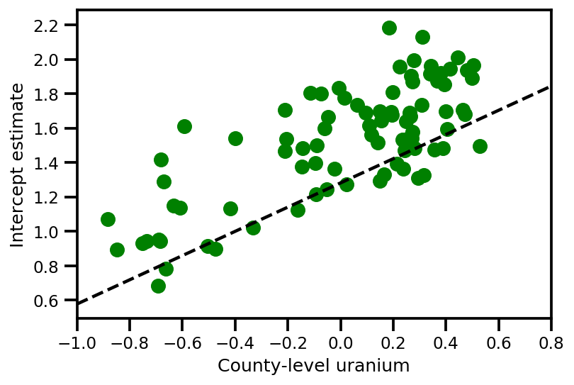
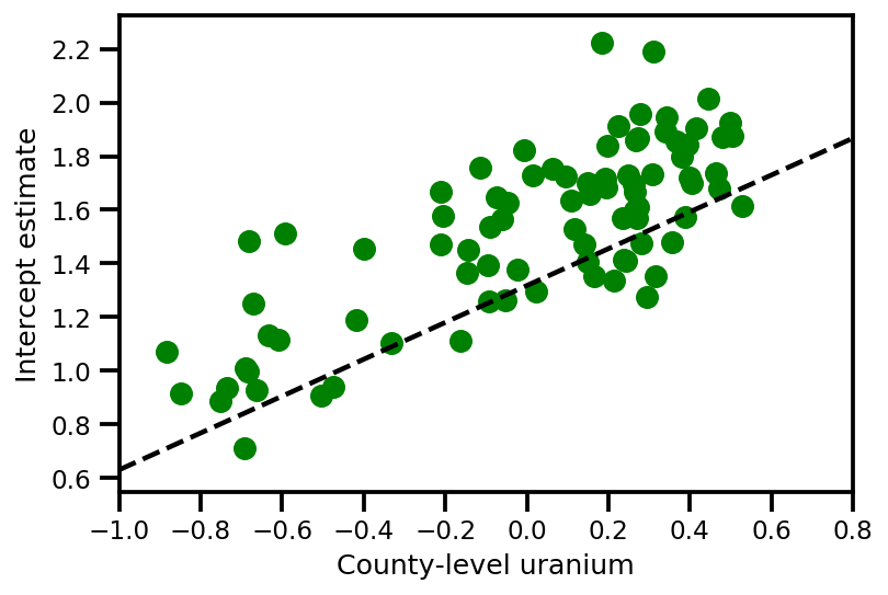
a_means = (approx_param['gamma']['mu'][0] 
         + approx_param['gamma']['mu'][1]*u.values
         + approx_param['gamma']['mu'][2]*xbar[county]
         + approx_param['eps']['mu'][county])
_, index = np.unique(county, return_index=True)
plt.scatter(u.values[index], a_means[index], color='g')

xvals = np.linspace(-1, 0.8)
plt.plot(xvals, 
         approx_param['gamma']['mu'][0]+approx_param['gamma']['mu'][1]*xvals, 
         'k--')
plt.xlim(-1, 0.8)

plt.xlabel('County-level uranium');
plt.ylabel('Intercept estimate');

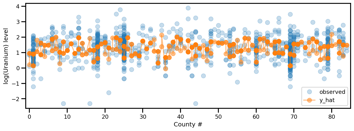
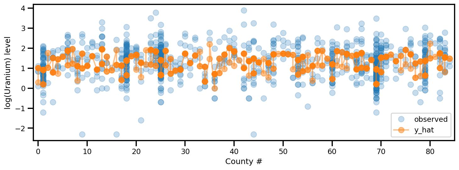
y_est = (approx_param['gamma']['mu'][0] 
        + approx_param['gamma']['mu'][1]*u.values
        + approx_param['gamma']['mu'][2]*xbar[county]
        + approx_param['eps']['mu'][county]
        + approx_param['b']['mu']*floor_measure)

_, ax = plt.subplots(1, 1, figsize=(12, 4))
ax.plot(county, log_radon, 'o', alpha=.25, label='observed')
ax.plot(county, y_est, '-o', lw=2, alpha=.5, label='y_hat')
ax.set_xlim(-1, county.max()+1)
plt.legend(loc='lower right')
ax.set_xlabel('County #')
ax.set_ylabel('log(Uranium) level');

FullRank ADVI

對於完整秩 ADVI，我們希望使用多變量高斯分佈來近似後驗。

USE_FULLRANK = True

*prior_tensors, _ = contextual_effect2.sample()

mapper = Mapper(prior_tensors,
                [tfb.Identity() for _ in prior_tensors],
                contextual_effect2.event_shape[:-1])

rv_shape = ps.shape(mapper.flatten_and_concat(mapper.list_of_tensors))
init_val = tf.random.normal(rv_shape, dtype=dtype)
loc = tf.Variable(init_val, name='loc', dtype=dtype)

if USE_FULLRANK:
  # cov_param = tfp.util.TransformedVariable(
  #     10. * tf.eye(rv_shape[0], dtype=dtype),
  #     tfb.FillScaleTriL(),
  #     name='cov_param'
  #     )
  FillScaleTriL = tfb.FillScaleTriL(
        diag_bijector=tfb.Chain([
          tfb.Shift(tf.cast(.01, dtype)),
          tfb.Softplus(),
          tfb.Shift(tf.cast(np.log(np.expm1(1.)), dtype))]),
        diag_shift=None)
  cov_param = tfp.util.TransformedVariable(
      .02 * tf.eye(rv_shape[0], dtype=dtype), 
      FillScaleTriL,
      name='cov_param')
  advi_approx = tfd.MultivariateNormalTriL(
      loc=loc, scale_tril=cov_param)
else:
  # An alternative way to build meanfield ADVI.
  cov_param = tfp.util.TransformedVariable(
      .02 * tf.ones(rv_shape, dtype=dtype),
      tfb.Softplus(),
      name='cov_param'
      )
  advi_approx = tfd.MultivariateNormalDiag(
      loc=loc, scale_diag=cov_param)

contextual_effect_posterior2 = lambda x: contextual_effect_posterior(
    *mapper.split_and_reshape(x)
)

# Check the logp and logq
advi_samples = advi_approx.sample(7)
pprint([
  advi_approx.log_prob(advi_samples),
  contextual_effect_posterior2(advi_samples)
  ])

[<tf.Tensor: shape=(7,), dtype=float64, numpy=
array([238.81841799, 217.71022639, 234.57207103, 230.0643819 ,
       243.73140943, 226.80149702, 232.85184209])>,
 <tf.Tensor: shape=(7,), dtype=float64, numpy=
array([-3638.93663169, -3664.25879314, -3577.69371677, -3696.25705312,
       -3689.12130489, -3777.53698383, -3659.4982734 ])>]

learning_rate = tf_keras.optimizers.schedules.ExponentialDecay(
    initial_learning_rate=1e-2,
    decay_steps=10,
    decay_rate=0.99,
    staircase=True)

opt = tf_keras.optimizers.Adam(learning_rate=learning_rate)

@tf.function(experimental_compile=True)
def run_approximation():
  loss_ = tfp.vi.fit_surrogate_posterior(
        contextual_effect_posterior2,
        surrogate_posterior=advi_approx,
        optimizer=opt,
        sample_size=10,
        num_steps=1000)
  return loss_

loss_ = run_approximation()

plt.plot(loss_);
plt.xlabel('iter');
plt.ylabel('loss');

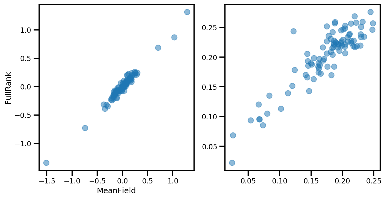
# debug
if True:
  _, ax = plt.subplots(1, 2, figsize=(10, 5))
  ax[0].plot(mapper.flatten_and_concat(advi.mean()), advi_approx.mean(), 'o', alpha=.5)
  ax[1].plot(mapper.flatten_and_concat(advi.stddev()), advi_approx.stddev(), 'o', alpha=.5)
  ax[0].set_xlabel('MeanField')
  ax[0].set_ylabel('FullRank')

graph_info = contextual_effect2.resolve_graph()
approx_param = dict()

free_param_mean = mapper.split_and_reshape(advi_approx.mean())
free_param_std = mapper.split_and_reshape(advi_approx.stddev())
for i, (rvname, param) in enumerate(graph_info[:-1]):
  approx_param[rvname] = {"mu": free_param_mean[i].numpy(),
                          "cov_info": free_param_std[i].numpy()}

a_means = (approx_param['gamma']['mu'][0] 
         + approx_param['gamma']['mu'][1]*u.values
         + approx_param['gamma']['mu'][2]*xbar[county]
         + approx_param['eps']['mu'][county])
_, index = np.unique(county, return_index=True)
plt.scatter(u.values[index], a_means[index], color='g')

xvals = np.linspace(-1, 0.8)
plt.plot(xvals, 
         approx_param['gamma']['mu'][0]+approx_param['gamma']['mu'][1]*xvals, 
         'k--')
plt.xlim(-1, 0.8)

plt.xlabel('County-level uranium');
plt.ylabel('Intercept estimate');

y_est = (approx_param['gamma']['mu'][0] 
         + approx_param['gamma']['mu'][1]*u.values
         + approx_param['gamma']['mu'][2]*xbar[county]
         + approx_param['eps']['mu'][county]
         + approx_param['b']['mu']*floor_measure)

_, ax = plt.subplots(1, 1, figsize=(12, 4))
ax.plot(county, log_radon, 'o', alpha=.25, label='observed')
ax.plot(county, y_est, '-o', lw=2, alpha=.5, label='y_hat')
ax.set_xlim(-1, county.max()+1)
plt.legend(loc='lower right')
ax.set_xlabel('County #')
ax.set_ylabel('log(Uranium) level');

Beta-Bernoulli 混合模型

一種混合模型，其中多位審查者標記某些項目，具有未知的（真實）潛在標籤。

dtype = tf.float32

n = 50000    # number of examples reviewed
p_bad_ = 0.1 # fraction of bad events
m = 5        # number of reviewers for each example
rcl_ = .35 + np.random.rand(m)/10
prc_ = .65 + np.random.rand(m)/10

# PARAMETER TRANSFORMATION
tpr = rcl_
fpr = p_bad_*tpr*(1./prc_-1.)/(1.-p_bad_)
tnr = 1 - fpr

# broadcast to m reviewer.
batch_prob = np.asarray([tpr, fpr]).T
mixture = tfd.Mixture(
    tfd.Categorical(
        probs=[p_bad_, 1-p_bad_]),
    [
        tfd.Independent(tfd.Bernoulli(probs=tpr), 1),
        tfd.Independent(tfd.Bernoulli(probs=fpr), 1),
    ])
# Generate reviewer response
X_tf = mixture.sample([n])

# run once to always use the same array as input
# so we can compare the estimation from different
# inference method.
X_np = X_tf.numpy()

# batched Mixture model
mdl_mixture = tfd.JointDistributionSequential([
    tfd.Sample(tfd.Beta(5., 2.), m),
    tfd.Sample(tfd.Beta(2., 2.), m),
    tfd.Sample(tfd.Beta(1., 10), 1),
    lambda p_bad, rcl, prc: tfd.Sample(
        tfd.Mixture(
            tfd.Categorical(
                probs=tf.concat([p_bad, 1.-p_bad], -1)),
            [
              tfd.Independent(tfd.Bernoulli(
                  probs=rcl), 1),
              tfd.Independent(tfd.Bernoulli(
                  probs=p_bad*rcl*(1./prc-1.)/(1.-p_bad)), 1)
             ]
      ), (n, )), 
    ])

mdl_mixture.resolve_graph()

(('prc', ()), ('rcl', ()), ('p_bad', ()), ('x', ('p_bad', 'rcl', 'prc')))

prc, rcl, p_bad, x = mdl_mixture.sample(4)
x.shape

TensorShape([4, 50000, 5])

mdl_mixture.log_prob_parts([prc, rcl, p_bad, X_np[np.newaxis, ...]])

[<tf.Tensor: shape=(4,), dtype=float32, numpy=array([1.4828572, 2.957961 , 2.9355168, 2.6116824], dtype=float32)>,
 <tf.Tensor: shape=(4,), dtype=float32, numpy=array([-0.14646745,  1.3308513 ,  1.1205603 ,  0.5441705 ], dtype=float32)>,
 <tf.Tensor: shape=(4,), dtype=float32, numpy=array([1.3733709, 1.8020535, 2.1865845, 1.5701319], dtype=float32)>,
 <tf.Tensor: shape=(4,), dtype=float32, numpy=array([-54326.664, -52683.93 , -64407.67 , -55007.895], dtype=float32)>]

推論 (NUTS)

nchain = 10
prc, rcl, p_bad, _ = mdl_mixture.sample(nchain)
initial_chain_state = [prc, rcl, p_bad]

# Since MCMC operates over unconstrained space, we need to transform the
# samples so they live in real-space.
unconstraining_bijectors = [
    tfb.Sigmoid(),       # Maps R to [0, 1].
    tfb.Sigmoid(),       # Maps R to [0, 1].
    tfb.Sigmoid(),       # Maps R to [0, 1].
]
step_size = [tf.cast(i, dtype=dtype) for i in [1e-3, 1e-3, 1e-3]]

X_expanded = X_np[np.newaxis, ...]
target_log_prob_fn = lambda *x: mdl_mixture.log_prob(x + (X_expanded, ))

samples, sampler_stat = run_chain(
    initial_chain_state, step_size, target_log_prob_fn, 
    unconstraining_bijectors, burnin=100)

# using the pymc3 naming convention
sample_stats_name = ['lp', 'tree_size', 'diverging', 'energy', 'mean_tree_accept']
sample_stats = {k:v.numpy().T for k, v in zip(sample_stats_name, sampler_stat)}
sample_stats['tree_size'] = np.diff(sample_stats['tree_size'], axis=1)

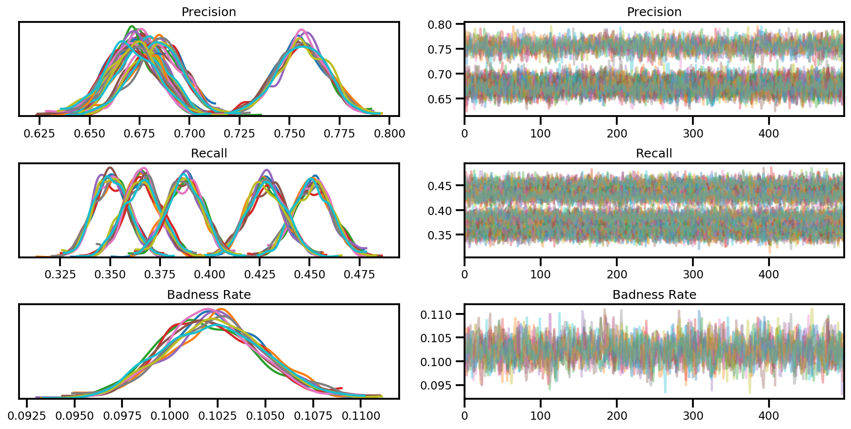
var_name = ['Precision', 'Recall', 'Badness Rate']
posterior = {k:np.swapaxes(v.numpy(), 1, 0) 
             for k, v in zip(var_name, samples)}

az_trace = az.from_dict(posterior=posterior, sample_stats=sample_stats)

axes = az.plot_trace(az_trace, compact=True);