
|
|
|
 在 GitHub 上檢視原始碼 在 GitHub 上檢視原始碼
|
|
安裝
安裝
摘要
在此 Colab 中,我們示範如何使用 TensorFlow Probability 中的變分推論來擬合廣義線性混合效應模型。
模型系列
廣義線性混合效應模型 (GLMM) 類似於廣義線性模型 (GLM),不同之處在於前者將樣本特定的雜訊納入預測的線性響應中。這在某些方面很有用,因為它允許鮮少出現的特徵與更常見的特徵共用資訊。
作為生成過程,廣義線性混合效應模型 (GLMM) 的特徵在於
\[ \begin{align} \text{for } & r = 1\ldots R: \hspace{2.45cm}\text{# 針對每個隨機效應群組}\\ &\begin{aligned} \text{for } &c = 1\ldots |C_r|: \hspace{1.3cm}\text{# 針對群組 $r$ 的每個類別 (「層級」)}\\ &\begin{aligned} \beta_{rc} &\sim \text{MultivariateNormal}(\text{loc}=0_{D_r}, \text{scale}=\Sigma_r^{1/2}) \end{aligned} \end{aligned}\\\\ \text{for } & i = 1 \ldots N: \hspace{2.45cm}\text{# 針對每個樣本}\\ &\begin{aligned} &\eta_i = \underbrace{\vphantom{\sum_{r=1}^R}x_i^\top\omega}_\text{固定效應} + \underbrace{\sum_{r=1}^R z_{r,i}^\top \beta_{r,C_r(i) } }_\text{隨機效應} \\ &Y_i|x_i,\omega,\{z_{r,i} , \beta_r\}_{r=1}^R \sim \text{Distribution}(\text{mean}= g^{-1}(\eta_i)) \end{aligned} \end{align} \]
其中
\[ \begin{align} R &= \text{隨機效應群組的數量}\\ |C_r| &= \text{群組 $r$ 的類別數量}\\ N &= \text{訓練樣本的數量}\\ x_i,\omega &\in \mathbb{R}^{D_0}\\ D_0 &= \text{固定效應的數量}\\ C_r(i) &= \text{第 $i$ 個樣本的類別 (在群組 $r$ 下)}\\ z_{r,i} &\in \mathbb{R}^{D_r}\\ D_r &= \text{與群組 $r$ 相關聯的隨機效應數量}\\ \Sigma_{r} &\in \{S\in\mathbb{R}^{D_r \times D_r} : S \succ 0 \}\\ \eta_i\mapsto g^{-1}(\eta_i) &= \mu_i, \text{反向連結函數}\\ \text{Distribution} &=\text{僅可透過其平均數參數化的某些分佈} \end{align} \]
換句話說,這表示每個群組的每個類別都與多變數常態分佈中的樣本 \(\beta_{rc}\) 相關聯。雖然 \(\beta_{rc}\) 繪圖始終是獨立的,但它們僅針對群組 \(r\) 進行相同分佈:請注意,每個 \(r\in\{1,\ldots,R\}\) 只有一個 \(\Sigma_r\)。
當與樣本群組的特徵 (\(z_{r,i}\)) 進行仿射組合時,結果是第 \(i\) 個預測線性響應上的樣本特定雜訊 (否則為 \(x_i^\top\omega\))。
當我們估計 \(\{\Sigma_r:r\in\{1,\ldots,R\}\}\) 時,我們基本上是在估計隨機效應群組攜帶的雜訊量,否則這些雜訊會淹沒 \(x_i^\top\omega\) 中存在的訊號。
對於 \(\text{Distribution}\) 和反向連結函數 \(g^{-1}\),有多種選項。常見的選項包括
- \(Y_i\sim\text{Normal}(\text{mean}=\eta_i, \text{scale}=\sigma)\),
- \(Y_i\sim\text{Binomial}(\text{mean}=n_i \cdot \text{sigmoid}(\eta_i), \text{total_count}=n_i)\),以及,
- \(Y_i\sim\text{Poisson}(\text{mean}=\exp(\eta_i))\)。
如需更多可能性,請參閱 tfp.glm 模組。
變分推論
遺憾的是,尋找參數 \(\beta,\{\Sigma_r\}_r^R\) 的最大概似估計需要進行非解析積分。為了規避這個問題,我們改為
- 定義參數化分佈系列 (「替代密度」),在附錄中表示為 \(q_{\lambda}\)。
- 尋找參數 \(\lambda\),使 \(q_{\lambda}\) 接近我們的真實目標密度。
分佈系列將是適當維度的獨立高斯分佈,而「接近我們的目標密度」是指「最小化 Kullback-Leibler 散度」。例如,請參閱 「變分推論:統計學家的評論」第 2.2 節,其中有詳細的推導和動機。特別是,它顯示最小化 K-L 散度等同於最小化負證據下界 (ELBO)。
玩具問題
Gelman 等人 (2007) 的「氡資料集」是一個有時用於示範迴歸方法的資料集。(例如,這個密切相關的 PyMC3 部落格文章。) 氡資料集包含在美國各地進行的室內氡測量值。氡是一種天然存在的放射性氣體,在高濃度下具有毒性。
對於我們的示範,假設我們有興趣驗證「在有地下室的家庭中,氡含量較高」的假設。我們也懷疑氡濃度與土壤類型有關,亦即地理位置很重要。
為了將此問題構建成 ML 問題,我們將嘗試根據讀數所在的樓層的線性函數來預測對數氡含量。我們也將使用郡作為隨機效應,並以此方式來解釋地理位置造成的變異數。換句話說,我們將使用廣義線性混合效應模型。
%matplotlib inline
%config InlineBackend.figure_format = 'retina'

import os
from six.moves import urllib

import matplotlib.pyplot as plt; plt.style.use('ggplot')
import numpy as np
import pandas as pd
import seaborn as sns; sns.set_context('notebook')
import tensorflow_datasets as tfds

import tensorflow as tf
import tf_keras

import tensorflow_probability as tfp
tfd = tfp.distributions
tfb = tfp.bijectors
我們也將快速檢查 GPU 的可用性
if tf.test.gpu_device_name() != '/device:GPU:0':
  print("We'll just use the CPU for this run.")
else:
  print('Huzzah! Found GPU: {}'.format(tf.test.gpu_device_name()))
We'll just use the CPU for this run.
取得資料集
我們從 TensorFlow 資料集載入資料集,並進行一些輕微的預先處理。
def load_and_preprocess_radon_dataset(state='MN'):
  """Load the Radon dataset from TensorFlow Datasets and preprocess it.

  Following the examples in "Bayesian Data Analysis" (Gelman, 2007), we filter
  to Minnesota data and preprocess to obtain the following features:
  - `county`: Name of county in which the measurement was taken.
  - `floor`: Floor of house (0 for basement, 1 for first floor) on which the
    measurement was taken.

  The target variable is `log_radon`, the log of the Radon measurement in the
  house.
  """
  ds = tfds.load('radon', split='train')
  radon_data = tfds.as_dataframe(ds)
  radon_data.rename(lambda s: s[9:] if s.startswith('feat') else s, axis=1, inplace=True)
  df = radon_data[radon_data.state==state.encode()].copy()

  df['radon'] = df.activity.apply(lambda x: x if x > 0. else 0.1)
  # Make county names look nice.
  df['county'] = df.county.apply(lambda s: s.decode()).str.strip().str.title()
  # Remap categories to start from 0 and end at max(category).
  df['county'] = df.county.astype(pd.api.types.CategoricalDtype())
  df['county_code'] = df.county.cat.codes
  # Radon levels are all positive, but log levels are unconstrained
  df['log_radon'] = df['radon'].apply(np.log)

  # Drop columns we won't use and tidy the index
  columns_to_keep = ['log_radon', 'floor', 'county', 'county_code']
  df = df[columns_to_keep].reset_index(drop=True)

  return df

df = load_and_preprocess_radon_dataset()
df.head()
專門化 GLMM 系列
在本節中,我們將 GLMM 系列專門化,以執行預測氡含量的任務。為此,我們先考慮 GLMM 的固定效應特殊情況
\[ \mathbb{E}[\log(\text{radon}_j)] = c + \text{floor_effect}_j \]
此模型假設觀察 \(j\) 中的對數氡 (在預期中) 受進行第 \(j\) 次讀數的樓層加上一些常數截距控制。在虛擬碼中,我們可能會寫成
def estimate_log_radon(floor):
    return intercept + floor_effect[floor]
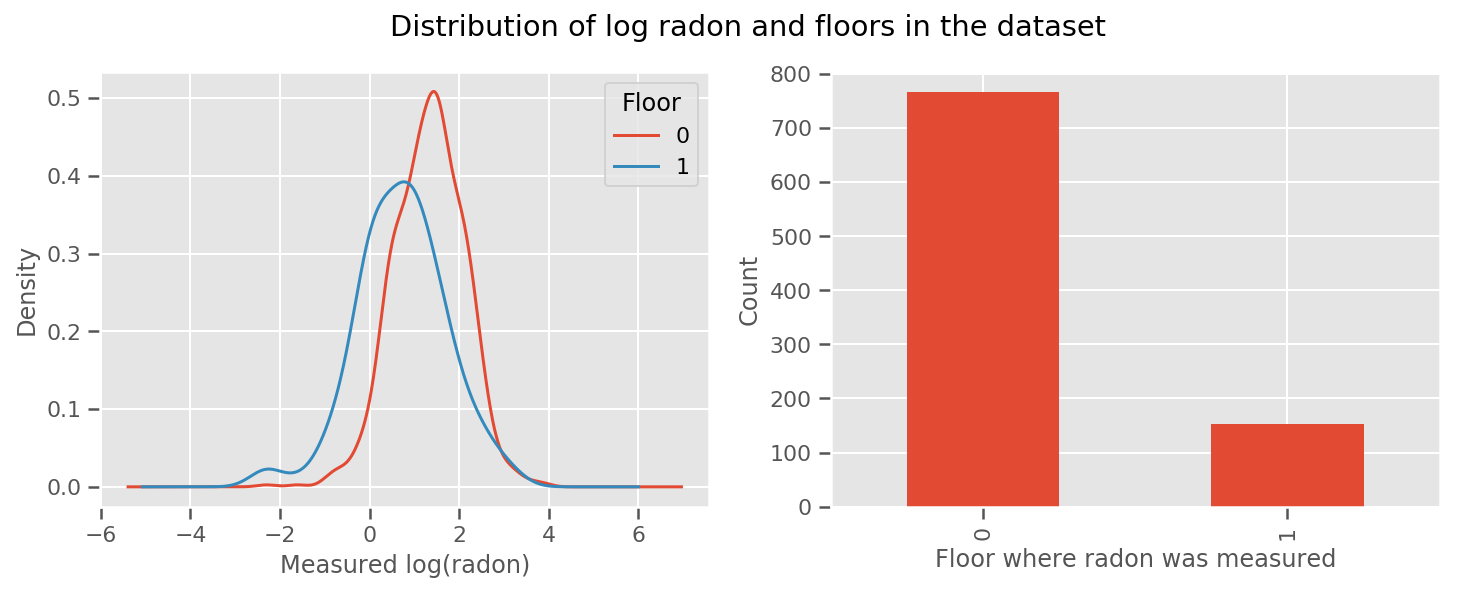
為每個樓層和通用 intercept 項學習權重。查看來自 0 樓和 1 樓的氡測量值,看起來這可能是一個好的開始
fig, (ax1, ax2) = plt.subplots(ncols=2, figsize=(12, 4))
df.groupby('floor')['log_radon'].plot(kind='density', ax=ax1);
ax1.set_xlabel('Measured log(radon)')
ax1.legend(title='Floor')

df['floor'].value_counts().plot(kind='bar', ax=ax2)
ax2.set_xlabel('Floor where radon was measured')
ax2.set_ylabel('Count')
fig.suptitle("Distribution of log radon and floors in the dataset");
為了使模型更加複雜,包括一些關於地理位置的資訊可能會更好:氡是鈾衰變鏈的一部分,鈾可能存在於地下,因此地理位置似乎是關鍵的考量因素。
\[ \mathbb{E}[\log(\text{radon}_j)] = c + \text{floor_effect}_j + \text{county_effect}_j \]
同樣,在虛擬碼中,我們有
def estimate_log_radon(floor, county):
    return intercept + floor_effect[floor] + county_effect[county]
與之前相同,只是使用了郡特定的權重。
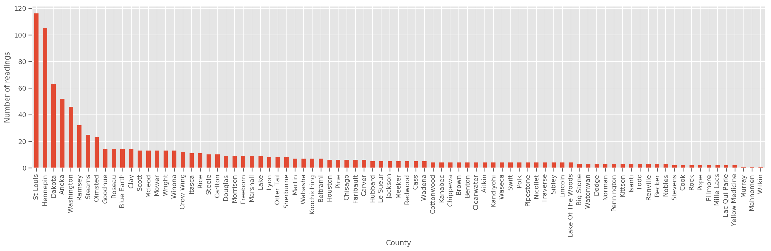
假設有足夠大的訓練集,這是一個合理的模型。但是,根據我們來自明尼蘇達州的資料,我們看到有大量郡的測量次數很少。例如,在 85 個郡中,有 39 個郡的觀察次數少於五次。
這促使我們在所有觀察值之間共用統計強度,使其在每個郡的觀察次數增加時收斂到上述模型。
fig, ax = plt.subplots(figsize=(22, 5));
county_freq = df['county'].value_counts()
county_freq.plot(kind='bar', ax=ax)
ax.set_xlabel('County')
ax.set_ylabel('Number of readings');
如果我們擬合此模型,則 county_effect 向量可能會最終記住僅具有少量訓練樣本的郡的結果,這可能會過度擬合並導致不良的泛化。
GLMM 為上述兩個 GLM 提供了一個令人滿意的中間方案。我們可以考慮擬合
\[ \log(\text{radon}_j) \sim c + \text{floor_effect}_j + \mathcal{N}(\text{county_effect}_j, \text{county_scale}) \]
此模型與第一個模型相同,但我們已將概似固定為常態分佈,並將透過 (單個) 變數 county_scale 在所有郡之間共用變異數。在虛擬碼中,
def estimate_log_radon(floor, county):
    county_mean = county_effect[county]
    random_effect = np.random.normal() * county_scale + county_mean
    return intercept + floor_effect[floor] + random_effect
我們將使用觀察到的資料來推斷 county_scale、county_mean 和 random_effect 的聯合分佈。全域 county_scale 允許我們在郡之間共用統計強度:具有許多觀察值的郡為觀察值少的郡的變異數提供點擊率。此外,隨著我們收集更多資料,此模型將收斂到沒有匯集尺度變數的模型 - 即使使用此資料集,對於觀察次數最多的郡,我們也會得出與任一模型相似的結論。
實驗
我們現在將嘗試在 TensorFlow 中使用變分推論來擬合上述 GLMM。首先,我們將資料分成特徵和標籤。
features = df[['county_code', 'floor']].astype(int)
labels = df[['log_radon']].astype(np.float32).values.flatten()
指定模型
def make_joint_distribution_coroutine(floor, county, n_counties, n_floors):

  def model():
    county_scale = yield tfd.HalfNormal(scale=1., name='scale_prior')
    intercept = yield tfd.Normal(loc=0., scale=1., name='intercept')
    floor_weight = yield tfd.Normal(loc=0., scale=1., name='floor_weight')
    county_prior = yield tfd.Normal(loc=tf.zeros(n_counties),
                                    scale=county_scale,
                                    name='county_prior')
    random_effect = tf.gather(county_prior, county, axis=-1)

    fixed_effect = intercept + floor_weight * floor
    linear_response = fixed_effect + random_effect
    yield tfd.Normal(loc=linear_response, scale=1., name='likelihood')
  return tfd.JointDistributionCoroutineAutoBatched(model)

joint = make_joint_distribution_coroutine(
    features.floor.values, features.county_code.values, df.county.nunique(),
    df.floor.nunique())

# Define a closure over the joint distribution
# to condition on the observed labels.
def target_log_prob_fn(*args):
  return joint.log_prob(*args, likelihood=labels)
指定替代後驗
現在,我們將替代系列 \(q_{\lambda}\) 放在一起,其中參數 \(\lambda\) 是可訓練的。在本例中,我們的系列是獨立的多變數常態分佈,每個參數一個,而 \(\lambda = \{(\mu_j, \sigma_j)\}\),其中 \(j\) 索引四個參數。
我們用於擬合替代系列的方法使用 tf.Variables。我們也使用 tfp.util.TransformedVariable 以及 Softplus 來約束 (可訓練的) 尺度參數為正數。此外,我們將 Softplus 應用於整個 scale_prior,這是一個正參數。
我們使用一些抖動來初始化這些可訓練的變數,以幫助進行最佳化。
# Initialize locations and scales randomly with `tf.Variable`s and
# `tfp.util.TransformedVariable`s.
_init_loc = lambda shape=(): tf.Variable(
    tf.random.uniform(shape, minval=-2., maxval=2.))
_init_scale = lambda shape=(): tfp.util.TransformedVariable(
    initial_value=tf.random.uniform(shape, minval=0.01, maxval=1.),
    bijector=tfb.Softplus())
n_counties = df.county.nunique()

surrogate_posterior = tfd.JointDistributionSequentialAutoBatched([
  tfb.Softplus()(tfd.Normal(_init_loc(), _init_scale())),           # scale_prior
  tfd.Normal(_init_loc(), _init_scale()),                           # intercept
  tfd.Normal(_init_loc(), _init_scale()),                           # floor_weight
  tfd.Normal(_init_loc([n_counties]), _init_scale([n_counties]))])  # county_prior
請注意,此儲存格可以替換為 tfp.experimental.vi.build_factored_surrogate_posterior,如下所示
surrogate_posterior = tfp.experimental.vi.build_factored_surrogate_posterior(
  event_shape=joint.event_shape_tensor()[:-1],
  constraining_bijectors=[tfb.Softplus(), None, None, None])
結果
回想一下,我們的目標是定義易於處理的參數化分佈系列,然後選擇參數,以便我們擁有一個接近我們目標分佈的易於處理的分佈。
我們已在上面建構了替代分佈,並且可以使用 tfp.vi.fit_surrogate_posterior,它接受最佳化工具和給定數量的步驟來尋找替代模型的參數,以最小化負 ELBO (這對應於最小化替代分佈和目標分佈之間的 Kullback-Liebler 散度)。
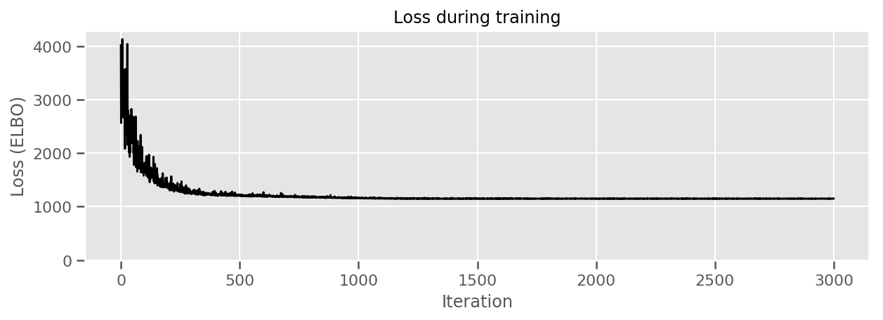
傳回值是每個步驟的負 ELBO,而 surrogate_posterior 中的分佈將已使用最佳化工具找到的參數進行更新。
optimizer = tf_keras.optimizers.Adam(learning_rate=1e-2)

losses = tfp.vi.fit_surrogate_posterior(
    target_log_prob_fn,
    surrogate_posterior,
    optimizer=optimizer,
    num_steps=3000,
    seed=42,
    sample_size=2)

(scale_prior_,
 intercept_,
 floor_weight_,
 county_weights_), _ = surrogate_posterior.sample_distributions()
print('        intercept (mean): ', intercept_.mean())
print('     floor_weight (mean): ', floor_weight_.mean())
print(' scale_prior (approx. mean): ', tf.reduce_mean(scale_prior_.sample(10000)))
intercept (mean):  tf.Tensor(1.4352839, shape=(), dtype=float32)
     floor_weight (mean):  tf.Tensor(-0.6701997, shape=(), dtype=float32)
 scale_prior (approx. mean):  tf.Tensor(0.28682157, shape=(), dtype=float32)
fig, ax = plt.subplots(figsize=(10, 3))
ax.plot(losses, 'k-')
ax.set(xlabel="Iteration",
       ylabel="Loss (ELBO)",
       title="Loss during training",
       ylim=0);
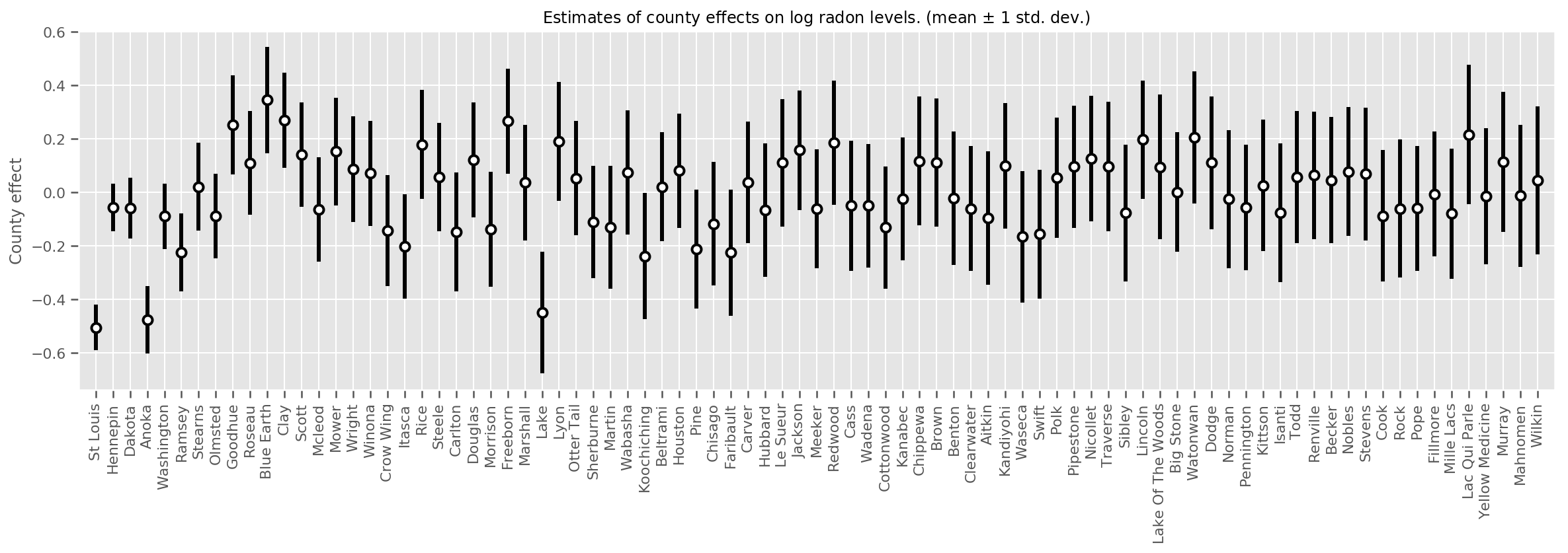
我們可以繪製估計的平均郡效應,以及該平均值的信賴區間。我們已按觀察次數對其進行排序,次數最多的在左側。請注意,對於觀察次數多的郡,信賴區間很小,但對於只有一次或兩次觀察值的郡,信賴區間較大。
county_counts = (df.groupby(by=['county', 'county_code'], observed=True)
                   .agg('size')
                   .sort_values(ascending=False)
                   .reset_index(name='count'))

means = county_weights_.mean()
stds = county_weights_.stddev()

fig, ax = plt.subplots(figsize=(20, 5))

for idx, row in county_counts.iterrows():
  mid = means[row.county_code]
  std = stds[row.county_code]
  ax.vlines(idx, mid - std, mid + std, linewidth=3)
  ax.plot(idx, means[row.county_code], 'ko', mfc='w', mew=2, ms=7)

ax.set(
    xticks=np.arange(len(county_counts)),
    xlim=(-1, len(county_counts)),
    ylabel="County effect",
    title=r"Estimates of county effects on log radon levels. (mean $\pm$ 1 std. dev.)",
)
ax.set_xticklabels(county_counts.county, rotation=90);
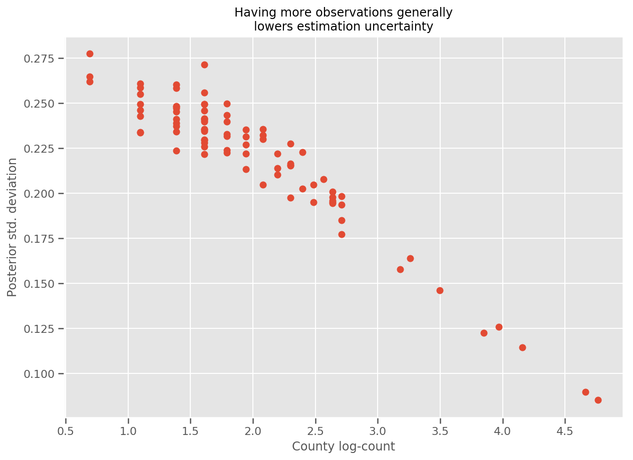
實際上,我們可以更直接地看到這一點,方法是繪製觀察次數的對數與估計標準差的關係圖,並看到該關係大致呈線性。
fig, ax = plt.subplots(figsize=(10, 7))
ax.plot(np.log1p(county_counts['count']), stds.numpy()[county_counts.county_code], 'o')
ax.set(
    ylabel='Posterior std. deviation',
    xlabel='County log-count',
    title='Having more observations generally\nlowers estimation uncertainty'
);
與 R 中的 lme4 比較
%%shell
exit  # Trick to make this block not execute.

radon = read.csv('srrs2.dat', header = TRUE)
radon = radon[radon$state=='MN',]
radon$radon = ifelse(radon$activity==0., 0.1, radon$activity)
radon$log_radon = log(radon$radon)

# install.packages('lme4')
library(lme4)
fit <- lmer(log_radon ~ 1 + floor + (1 | county), data=radon)
fit

# Linear mixed model fit by REML ['lmerMod']
# Formula: log_radon ~ 1 + floor + (1 | county)
#    Data: radon
# REML criterion at convergence: 2171.305
# Random effects:
#  Groups   Name        Std.Dev.
#  county   (Intercept) 0.3282
#  Residual             0.7556
# Number of obs: 919, groups:  county, 85
# Fixed Effects:
# (Intercept)        floor
#       1.462       -0.693
<IPython.core.display.Javascript at 0x7f90b888e9b0>
<IPython.core.display.Javascript at 0x7f90b888e780>
<IPython.core.display.Javascript at 0x7f90b888e780>
<IPython.core.display.Javascript at 0x7f90bce1dfd0>
<IPython.core.display.Javascript at 0x7f90b888e780>
<IPython.core.display.Javascript at 0x7f90b888e780>
<IPython.core.display.Javascript at 0x7f90b888e780>
<IPython.core.display.Javascript at 0x7f90b888e780>
下表總結了結果。
print(pd.DataFrame(data=dict(intercept=[1.462, tf.reduce_mean(intercept_.mean()).numpy()],
                             floor=[-0.693, tf.reduce_mean(floor_weight_.mean()).numpy()],
                             scale=[0.3282, tf.reduce_mean(scale_prior_.sample(10000)).numpy()]),
                   index=['lme4', 'vi']))
intercept   floor     scale
lme4   1.462000 -0.6930  0.328200
vi     1.435284 -0.6702  0.287251
此表表示 VI 結果在 lme4 的 ~10% 範圍內。這有點令人驚訝,因為
lme4基於 Laplace 方法 (而非 VI),- 在此 Colab 中未努力實際收斂,
- 在調整超參數方面僅做了極少努力,
- 未努力正規化或預先處理資料 (例如,居中特徵等)。
結論
在此 Colab 中,我們描述了廣義線性混合效應模型,並展示瞭如何使用變分推論,以使用 TensorFlow Probability 擬合這些模型。雖然玩具問題只有數百個訓練樣本,但此處使用的技術與大規模所需技術相同。