
|
|
|
 在 GitHub 上檢視來源 在 GitHub 上檢視來源
|
|
1 簡介
在這個 Colab 中,我們將把線性混合效應迴歸模型擬合到廣受歡迎的玩具資料集。我們將使用 R 的 lme4、Stan 的混合效應套件和 TensorFlow Probability (TFP) 基本元素進行三次擬合。最後,我們將展示這三者都給出大致相同的擬合參數和後驗分配。
我們的主要結論是,TFP 具有擬合 HLM 類模型的通用組件,並且它產生的結果與其他軟體套件(即 lme4、rstanarm)一致。這個 Colab 並未準確反映所比較的任何套件的計算效率。
%matplotlib inline

import os
from six.moves import urllib
import numpy as np
import pandas as pd
import warnings

from matplotlib import pyplot as plt
import seaborn as sns

from IPython.core.pylabtools import figsize
figsize(11, 9)

import tensorflow.compat.v1 as tf
import tensorflow_datasets as tfds
import tensorflow_probability as tfp
2 階層式線性模型
為了比較 R、Stan 和 TFP,我們將把階層式線性模型 (HLM) 擬合到 Radon 資料集,該資料集在 Gelman 等人所著的貝氏資料分析 中廣為人知(第二版第 559 頁;第三版第 250 頁)。
我們假設以下生成模型
\[\begin{align*} \text{for } & c=1\ldots \text{NumCounties}:\\ & \beta_c \sim \text{Normal}\left(\text{loc}=0, \text{scale}=\sigma_C \right) \\ \text{for } & i=1\ldots \text{NumSamples}:\\ &\eta_i = \underbrace{\omega_0 + \omega_1 \text{Floor}_i}_\text{固定效應} + \underbrace{\beta_{ \text{County}_i} \log( \text{UraniumPPM}_{\text{County}_i}))}_\text{隨機效應} \\ &\log(\text{Radon}_i) \sim \text{Normal}(\text{loc}=\eta_i , \text{scale}=\sigma_N) \end{align*}\]
在 R 的 lme4「波浪符號表示法」中,此模型等效於
log_radon ~ 1 + floor + (0 + log_uranium_ppm | county)
我們將使用 \({\beta_c\}_{c=1}^\text{NumCounties}\) 的後驗分配(以證據為條件)尋找 \(\omega, \sigma_C, \sigma_N\) 的 MLE。
如需基本上相同的模型,但具有隨機截距,請參閱附錄 A。
如需更通用的 HLM 規格,請參閱附錄 B。
3 資料整理
在本節中,我們取得 radon 資料集,並進行一些最少的預先處理,使其符合我們假設的模型。
def load_and_preprocess_radon_dataset(state='MN'):
  """Preprocess Radon dataset as done in "Bayesian Data Analysis" book.

  We filter to Minnesota data (919 examples) and preprocess to obtain the
  following features:
  - `log_uranium_ppm`: Log of soil uranium measurements.
  - `county`: Name of county in which the measurement was taken.
  - `floor`: Floor of house (0 for basement, 1 for first floor) on which the
    measurement was taken.

  The target variable is `log_radon`, the log of the Radon measurement in the
  house.
  """
  ds = tfds.load('radon', split='train')
  radon_data = tfds.as_dataframe(ds)
  radon_data.rename(lambda s: s[9:] if s.startswith('feat') else s, axis=1, inplace=True)
  df = radon_data[radon_data.state==state.encode()].copy()

  # For any missing or invalid activity readings, we'll use a value of `0.1`.
  df['radon'] = df.activity.apply(lambda x: x if x > 0. else 0.1)
  # Make county names look nice.
  df['county'] = df.county.apply(lambda s: s.decode()).str.strip().str.title()
  # Remap categories to start from 0 and end at max(category).
  county_name = sorted(df.county.unique())
  df['county'] = df.county.astype(
      pd.api.types.CategoricalDtype(categories=county_name)).cat.codes
  county_name = list(map(str.strip, county_name))

  df['log_radon'] = df['radon'].apply(np.log)
  df['log_uranium_ppm'] = df['Uppm'].apply(np.log)
  df = df[['idnum', 'log_radon', 'floor', 'county', 'log_uranium_ppm']]

  return df, county_name
radon, county_name = load_and_preprocess_radon_dataset()
# We'll use the following directory to store our preprocessed dataset.
CACHE_DIR = os.path.join(os.sep, 'tmp', 'radon')

# Save processed data. (So we can later read it in R.)
if not tf.gfile.Exists(CACHE_DIR):
  tf.gfile.MakeDirs(CACHE_DIR)
with tf.gfile.Open(os.path.join(CACHE_DIR, 'radon.csv'), 'w') as f:
  radon.to_csv(f, index=False)
3.1 瞭解您的資料
在本節中,我們探索 radon 資料集,以更好地瞭解為什麼提出的模型可能合理。
radon.head()
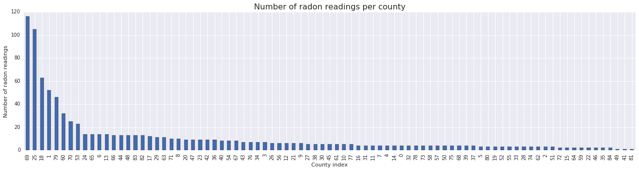
fig, ax = plt.subplots(figsize=(22, 5));
county_freq = radon['county'].value_counts()
county_freq.plot(kind='bar', color='#436bad');
plt.xlabel('County index')
plt.ylabel('Number of radon readings')
plt.title('Number of radon readings per county', fontsize=16)
county_freq = np.array(zip(county_freq.index, county_freq.values))  # We'll use this later.
fig, ax = plt.subplots(ncols=2, figsize=[10, 4]);

radon['log_radon'].plot(kind='density', ax=ax[0]);
ax[0].set_xlabel('log(radon)')

radon['floor'].value_counts().plot(kind='bar', ax=ax[1]);
ax[1].set_xlabel('Floor');
ax[1].set_ylabel('Count');

fig.subplots_adjust(wspace=0.25)
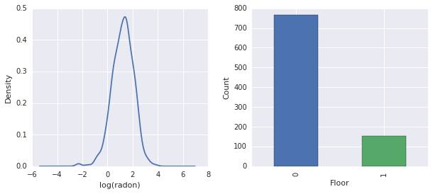
結論
- 有 85 個郡的長尾。(GLMM 中常見的情況。)
- 事實上,\(\log(\text{Radon})\) 是不受約束的。(因此線性迴歸可能合理。)
- 讀數大多在 \(0\) 樓進行;沒有在 \(1\) 樓以上進行讀數。(因此我們的固定效應將只有兩個權重。)
4 R 中的 HLM
在本節中,我們使用 R 的 lme4 套件來擬合上述機率模型。
suppressMessages({
  library('bayesplot')
  library('data.table')
  library('dplyr')
  library('gfile')
  library('ggplot2')
  library('lattice')
  library('lme4')
  library('plyr')
  library('rstanarm')
  library('tidyverse')
  RequireInitGoogle()
})
data = read_csv(gfile::GFile('/tmp/radon/radon.csv'))
Parsed with column specification:
cols(
  log_radon = col_double(),
  floor = col_integer(),
  county = col_integer(),
  log_uranium_ppm = col_double()
)
head(data)
# A tibble: 6 x 4
  log_radon floor county log_uranium_ppm
      <dbl> <int>  <int>           <dbl>
1     0.788     1      0          -0.689
2     0.788     0      0          -0.689
3     1.06      0      0          -0.689
4     0         0      0          -0.689
5     1.13      0      1          -0.847
6     0.916     0      1          -0.847
# https://github.com/stan-dev/example-models/wiki/ARM-Models-Sorted-by-Chapter
radon.model <- lmer(log_radon ~ 1 + floor  + (0 + log_uranium_ppm | county), data = data)
summary(radon.model)
Linear mixed model fit by REML ['lmerMod']
Formula: log_radon ~ 1 + floor + (0 + log_uranium_ppm | county)
   Data: data

REML criterion at convergence: 2166.3

Scaled residuals:
    Min      1Q  Median      3Q     Max
-4.5202 -0.6064  0.0107  0.6334  3.4111

Random effects:
 Groups   Name            Variance Std.Dev.
 county   log_uranium_ppm 0.7545   0.8686
 Residual                 0.5776   0.7600
Number of obs: 919, groups:  county, 85

Fixed effects:
            Estimate Std. Error t value
(Intercept)  1.47585    0.03899   37.85
floor       -0.67974    0.06963   -9.76

Correlation of Fixed Effects:
      (Intr)
floor -0.330
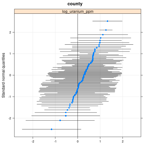
qqmath(ranef(radon.model, condVar=TRUE))
$county
write.csv(as.data.frame(ranef(radon.model, condVar = TRUE)), '/tmp/radon/lme4_fit.csv')
5 Stan 中的 HLM
在本節中,我們使用 rstanarm,使用與上述 lme4 模型相同的公式/語法來擬合 Stan 模型。
與 lme4 和下方的 TF 模型不同,rstanarm 是完全貝氏模型,也就是說,所有參數都被假定為從常態分配中抽取,而參數本身是從分配中抽取的。
fit <- stan_lmer(log_radon ~ 1 + floor + (0 + log_uranium_ppm | county), data = data)
SAMPLING FOR MODEL 'continuous' NOW (CHAIN 1).

Chain 1, Iteration:    1 / 2000 [  0%]  (Warmup)
Chain 1, Iteration:  200 / 2000 [ 10%]  (Warmup)
Chain 1, Iteration:  400 / 2000 [ 20%]  (Warmup)
Chain 1, Iteration:  600 / 2000 [ 30%]  (Warmup)
Chain 1, Iteration:  800 / 2000 [ 40%]  (Warmup)
Chain 1, Iteration: 1000 / 2000 [ 50%]  (Warmup)
Chain 1, Iteration: 1001 / 2000 [ 50%]  (Sampling)
Chain 1, Iteration: 1200 / 2000 [ 60%]  (Sampling)
Chain 1, Iteration: 1400 / 2000 [ 70%]  (Sampling)
Chain 1, Iteration: 1600 / 2000 [ 80%]  (Sampling)
Chain 1, Iteration: 1800 / 2000 [ 90%]  (Sampling)
Chain 1, Iteration: 2000 / 2000 [100%]  (Sampling)
 Elapsed Time: 7.73495 seconds (Warm-up)
               2.98852 seconds (Sampling)
               10.7235 seconds (Total)


SAMPLING FOR MODEL 'continuous' NOW (CHAIN 2).

Chain 2, Iteration:    1 / 2000 [  0%]  (Warmup)
Chain 2, Iteration:  200 / 2000 [ 10%]  (Warmup)
Chain 2, Iteration:  400 / 2000 [ 20%]  (Warmup)
Chain 2, Iteration:  600 / 2000 [ 30%]  (Warmup)
Chain 2, Iteration:  800 / 2000 [ 40%]  (Warmup)
Chain 2, Iteration: 1000 / 2000 [ 50%]  (Warmup)
Chain 2, Iteration: 1001 / 2000 [ 50%]  (Sampling)
Chain 2, Iteration: 1200 / 2000 [ 60%]  (Sampling)
Chain 2, Iteration: 1400 / 2000 [ 70%]  (Sampling)
Chain 2, Iteration: 1600 / 2000 [ 80%]  (Sampling)
Chain 2, Iteration: 1800 / 2000 [ 90%]  (Sampling)
Chain 2, Iteration: 2000 / 2000 [100%]  (Sampling)
 Elapsed Time: 7.51252 seconds (Warm-up)
               3.08653 seconds (Sampling)
               10.5991 seconds (Total)


SAMPLING FOR MODEL 'continuous' NOW (CHAIN 3).

Chain 3, Iteration:    1 / 2000 [  0%]  (Warmup)
Chain 3, Iteration:  200 / 2000 [ 10%]  (Warmup)
Chain 3, Iteration:  400 / 2000 [ 20%]  (Warmup)
Chain 3, Iteration:  600 / 2000 [ 30%]  (Warmup)
Chain 3, Iteration:  800 / 2000 [ 40%]  (Warmup)
Chain 3, Iteration: 1000 / 2000 [ 50%]  (Warmup)
Chain 3, Iteration: 1001 / 2000 [ 50%]  (Sampling)
Chain 3, Iteration: 1200 / 2000 [ 60%]  (Sampling)
Chain 3, Iteration: 1400 / 2000 [ 70%]  (Sampling)
Chain 3, Iteration: 1600 / 2000 [ 80%]  (Sampling)
Chain 3, Iteration: 1800 / 2000 [ 90%]  (Sampling)
Chain 3, Iteration: 2000 / 2000 [100%]  (Sampling)
 Elapsed Time: 8.14628 seconds (Warm-up)
               3.01001 seconds (Sampling)
               11.1563 seconds (Total)


SAMPLING FOR MODEL 'continuous' NOW (CHAIN 4).

Chain 4, Iteration:    1 / 2000 [  0%]  (Warmup)
Chain 4, Iteration:  200 / 2000 [ 10%]  (Warmup)
Chain 4, Iteration:  400 / 2000 [ 20%]  (Warmup)
Chain 4, Iteration:  600 / 2000 [ 30%]  (Warmup)
Chain 4, Iteration:  800 / 2000 [ 40%]  (Warmup)
Chain 4, Iteration: 1000 / 2000 [ 50%]  (Warmup)
Chain 4, Iteration: 1001 / 2000 [ 50%]  (Sampling)
Chain 4, Iteration: 1200 / 2000 [ 60%]  (Sampling)
Chain 4, Iteration: 1400 / 2000 [ 70%]  (Sampling)
Chain 4, Iteration: 1600 / 2000 [ 80%]  (Sampling)
Chain 4, Iteration: 1800 / 2000 [ 90%]  (Sampling)
Chain 4, Iteration: 2000 / 2000 [100%]  (Sampling)
 Elapsed Time: 7.6801 seconds (Warm-up)
               3.23663 seconds (Sampling)
               10.9167 seconds (Total)
fit
stan_lmer(formula = log_radon ~ 1 + floor + (0 + log_uranium_ppm |
    county), data = data)

Estimates:
            Median MAD_SD
(Intercept)  1.5    0.0
floor       -0.7    0.1
sigma        0.8    0.0

Error terms:
 Groups   Name            Std.Dev.
 county   log_uranium_ppm 0.87
 Residual                 0.76
Num. levels: county 85

Sample avg. posterior predictive
distribution of y (X = xbar):
         Median MAD_SD
mean_PPD 1.2    0.0

Observations: 919  Number of unconstrained parameters: 90
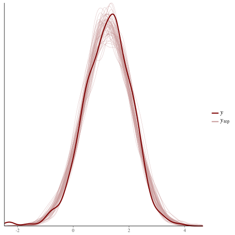
color_scheme_set("red")
ppc_dens_overlay(y = fit$y,
                 yrep = posterior_predict(fit, draws = 50))
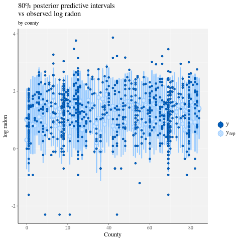
color_scheme_set("brightblue")
ppc_intervals(
  y = data$log_radon,
  yrep = posterior_predict(fit),
  x = data$county,
  prob = 0.8
) +
  labs(
    x = "County",
    y = "log radon",
    title = "80% posterior predictive intervals \nvs observed log radon",
    subtitle = "by county"
  ) +
  panel_bg(fill = "gray95", color = NA) +
  grid_lines(color = "white")
# Write the posterior samples (4000 for each variable) to a CSV.
write.csv(tidy(as.matrix(fit)), "/tmp/radon/stan_fit.csv")
with tf.gfile.Open('/tmp/radon/lme4_fit.csv', 'r') as f:
  lme4_fit = pd.read_csv(f, index_col=0)
lme4_fit.head()
從 lme4 擷取群組隨機效應的點估計值和條件標準差,以供稍後視覺化。
posterior_random_weights_lme4 = np.array(lme4_fit.condval, dtype=np.float32)
lme4_prior_scale = np.array(lme4_fit.condsd, dtype=np.float32)
print(posterior_random_weights_lme4.shape, lme4_prior_scale.shape)
(85,) (85,)
使用 lme4 估計的平均數和標準差,繪製郡權重的樣本。
with tf.Session() as sess:
  lme4_dist = tfp.distributions.Independent(
      tfp.distributions.Normal(
          loc=posterior_random_weights_lme4,
          scale=lme4_prior_scale),
      reinterpreted_batch_ndims=1)
  posterior_random_weights_lme4_final_ = sess.run(lme4_dist.sample(4000))
posterior_random_weights_lme4_final_.shape
(4000, 85)
我們也從 Stan 擬合中擷取郡權重的後驗樣本。
with tf.gfile.Open('/tmp/radon/stan_fit.csv', 'r') as f:
  samples = pd.read_csv(f, index_col=0)
samples.head()
posterior_random_weights_cols = [
    col for col in samples.columns if 'b.log_uranium_ppm.county' in col
]
posterior_random_weights_final_stan = samples[
    posterior_random_weights_cols].values
print(posterior_random_weights_final_stan.shape)
(4000, 85)
這個 Stan 範例 說明如何以更接近 TFP 的樣式實作 LMER,也就是直接指定機率模型。
6 TF Probability 中的 HLM
在本節中,我們將使用低階 TensorFlow Probability 基本元素 (Distributions) 來指定我們的階層式線性模型,並擬合未知的參數。
# Handy snippet to reset the global graph and global session.
with warnings.catch_warnings():
  warnings.simplefilter('ignore')
  tf.reset_default_graph()
  try:
    sess.close()
  except:
    pass
  sess = tf.InteractiveSession()
6.1 指定模型
在本節中,我們使用 TFP 基本元素指定 氡線性混合效應模型。為了做到這一點,我們指定兩個產生兩個 TFP 分配的函式
make_weights_prior:隨機權重的多變量常態先驗(乘以 \(\log(\text{UraniumPPM}_{c_i})\) 以計算線性預測值)。make_log_radon_likelihood:每個觀察到的 \(\log(\text{Radon}_i)\) 應變數上的Normal分配批次。
由於我們將擬合這些分配中每個分配的參數,因此我們必須使用 TF 變數(即 tf.get_variable)。但是,由於我們希望使用不受約束的最佳化,因此我們必須找到一種約束實值的方法,以實現必要的語意,例如,代表標準差的正數。
inv_scale_transform = lambda y: np.log(y)  # Not using TF here.
fwd_scale_transform = tf.exp
以下函式建構我們的先驗 \(p(\beta|\sigma_C)\),其中 \(\beta\) 表示隨機效應權重,\(\sigma_C\) 表示標準差。
我們使用 tf.make_template 來確保第一次呼叫此函式會實例化它使用的 TF 變數,而所有後續呼叫都會重複使用變數的目前值。
def _make_weights_prior(num_counties, dtype):
  """Returns a `len(log_uranium_ppm)` batch of univariate Normal."""
  raw_prior_scale = tf.get_variable(
      name='raw_prior_scale',
      initializer=np.array(inv_scale_transform(1.), dtype=dtype))
  return tfp.distributions.Independent(
      tfp.distributions.Normal(
          loc=tf.zeros(num_counties, dtype=dtype),
          scale=fwd_scale_transform(raw_prior_scale)),
      reinterpreted_batch_ndims=1)


make_weights_prior = tf.make_template(
    name_='make_weights_prior', func_=_make_weights_prior)
以下函式建構我們的概似 \(p(y|x,\omega,\beta,\sigma_N)\),其中 \(y,x\) 表示回應和證據,\(\omega,\beta\) 表示固定效應和隨機效應權重,而 \(\sigma_N\) 表示標準差。
在這裡,我們再次使用 tf.make_template 來確保 TF 變數在跨呼叫時重複使用。
def _make_log_radon_likelihood(random_effect_weights, floor, county,
                               log_county_uranium_ppm, init_log_radon_stddev):
  raw_likelihood_scale = tf.get_variable(
      name='raw_likelihood_scale',
      initializer=np.array(
          inv_scale_transform(init_log_radon_stddev), dtype=dtype))
  fixed_effect_weights = tf.get_variable(
      name='fixed_effect_weights', initializer=np.array([0., 1.], dtype=dtype))
  fixed_effects = fixed_effect_weights[0] + fixed_effect_weights[1] * floor
  random_effects = tf.gather(
      random_effect_weights * log_county_uranium_ppm,
      indices=tf.to_int32(county),
      axis=-1)
  linear_predictor = fixed_effects + random_effects
  return tfp.distributions.Normal(
      loc=linear_predictor, scale=fwd_scale_transform(raw_likelihood_scale))


make_log_radon_likelihood = tf.make_template(
    name_='make_log_radon_likelihood', func_=_make_log_radon_likelihood)
最後,我們使用先驗和概似產生器來建構聯合對數密度。
def joint_log_prob(random_effect_weights, log_radon, floor, county,
                   log_county_uranium_ppm, dtype):
  num_counties = len(log_county_uranium_ppm)
  rv_weights = make_weights_prior(num_counties, dtype)
  rv_radon = make_log_radon_likelihood(
      random_effect_weights,
      floor,
      county,
      log_county_uranium_ppm,
      init_log_radon_stddev=radon.log_radon.values.std())
  return (rv_weights.log_prob(random_effect_weights)
          + tf.reduce_sum(rv_radon.log_prob(log_radon), axis=-1))
6.2 訓練(期望值最大化演算法的隨機近似值)
為了擬合線性混合效應迴歸模型,我們將使用期望值最大化演算法 (SAEM) 的隨機近似值版本。基本概念是使用後驗樣本來近似預期的聯合對數密度(E 步驟)。然後,我們找到最大化此計算的參數(M 步驟)。更具體地說,定點迭代由下式給出
\[\begin{align*} \text{E}[ \log p(x, Z | \theta) | \theta_0] &\approx \frac{1}{M} \sum_{m=1}^M \log p(x, z_m | \theta), \quad Z_m\sim p(Z | x, \theta_0) && \text{E 步驟}\\ &=: Q_M(\theta, \theta_0) \\ \theta_0 &= \theta_0 - \eta \left.\nabla_\theta Q_M(\theta, \theta_0)\right|_{\theta=\theta_0} && \text{M 步驟} \end{align*}\]
其中 \(x\) 表示證據,\(Z\) 表示需要邊緣化的某些潛在變數,而 \(\theta,\theta_0\) 表示可能的參數化。
如需更詳盡的說明,請參閱 Bernard Delyon、Marc Lavielle、Eric、Moulines 所著的EM 演算法隨機近似值版本的收斂性 (Ann. Statist., 1999)。
為了計算 E 步驟,我們需要從後驗取樣。由於我們的後驗不容易取樣,因此我們使用漢彌爾頓蒙地卡羅法 (HMC)。HMC 是一種蒙地卡羅馬可夫鏈程序,它使用未正規化後驗對數密度的梯度(相對於狀態,而非參數)來提出新的樣本。
指定未正規化後驗對數密度很簡單,它僅僅是「固定」在我們希望條件化的任何事物的聯合對數密度。
# Specify unnormalized posterior.

dtype = np.float32

log_county_uranium_ppm = radon[
    ['county', 'log_uranium_ppm']].drop_duplicates().values[:, 1]
log_county_uranium_ppm = log_county_uranium_ppm.astype(dtype)

def unnormalized_posterior_log_prob(random_effect_weights):
  return joint_log_prob(
      random_effect_weights=random_effect_weights,
      log_radon=dtype(radon.log_radon.values),
      floor=dtype(radon.floor.values),
      county=np.int32(radon.county.values),
      log_county_uranium_ppm=log_county_uranium_ppm,
      dtype=dtype)
我們現在透過建立 HMC 轉換核心來完成 E 步驟設定。
注意事項
我們使用
state_stop_gradient=True來防止 M 步驟透過 MCMC 的繪製進行反向傳播。(回想一下,我們不需要透過反向傳播,因為我們的 E 步驟有意地在先前最知名的估計器中參數化。)我們使用
tf.placeholder,以便當我們最終執行 TF 圖時,我們可以將先前迭代的隨機 MCMC 樣本饋送為下一次迭代的鏈值。我們使用 TFP 的自適應
step_size啟發式演算法tfp.mcmc.hmc_step_size_update_fn。
# Set-up E-step.

step_size = tf.get_variable(
    'step_size',
    initializer=np.array(0.2, dtype=dtype),
    trainable=False)

hmc = tfp.mcmc.HamiltonianMonteCarlo(
    target_log_prob_fn=unnormalized_posterior_log_prob,
    num_leapfrog_steps=2,
    step_size=step_size,
    step_size_update_fn=tfp.mcmc.make_simple_step_size_update_policy(
      num_adaptation_steps=None),
    state_gradients_are_stopped=True)

init_random_weights = tf.placeholder(dtype, shape=[len(log_county_uranium_ppm)])

posterior_random_weights, kernel_results = tfp.mcmc.sample_chain(
    num_results=3,
    num_burnin_steps=0,
    num_steps_between_results=0,
    current_state=init_random_weights,
    kernel=hmc)
我們現在設定 M 步驟。這基本上與人們在 TF 中可能執行的最佳化相同。
# Set-up M-step.

loss = -tf.reduce_mean(kernel_results.accepted_results.target_log_prob)

global_step = tf.train.get_or_create_global_step()

learning_rate = tf.train.exponential_decay(
    learning_rate=0.1,
    global_step=global_step,
    decay_steps=2,
    decay_rate=0.99)

optimizer = tf.train.AdamOptimizer(learning_rate=learning_rate)
train_op = optimizer.minimize(loss, global_step=global_step)
最後,我們完成一些內務處理任務。我們必須告訴 TF 所有變數都已初始化。我們也建立 TF 變數的控制代碼,以便我們可以在程序的每次迭代中 print 其值。
# Initialize all variables.

init_op = tf.initialize_all_variables()
# Grab variable handles for diagnostic purposes.

with tf.variable_scope('make_weights_prior', reuse=True):
  prior_scale = fwd_scale_transform(tf.get_variable(
      name='raw_prior_scale', dtype=dtype))

with tf.variable_scope('make_log_radon_likelihood', reuse=True):
  likelihood_scale = fwd_scale_transform(tf.get_variable(
      name='raw_likelihood_scale', dtype=dtype))
  fixed_effect_weights = tf.get_variable(
      name='fixed_effect_weights', dtype=dtype)
6.3 執行
在本節中,我們執行 SAEM TF 圖。這裡的主要技巧是將我們從 HMC 核心的最後一次繪製饋送到下一次迭代中。這是透過在 sess.run 呼叫中使用 feed_dict 來實現的。
init_op.run()
w_ = np.zeros([len(log_county_uranium_ppm)], dtype=dtype)
%%time
maxiter = int(1500)
num_accepted = 0
num_drawn = 0
for i in range(maxiter):
  [
      _,
      global_step_,
      loss_,
      posterior_random_weights_,
      kernel_results_,
      step_size_,
      prior_scale_,
      likelihood_scale_,
      fixed_effect_weights_,
  ] = sess.run([
      train_op,
      global_step,
      loss,
      posterior_random_weights,
      kernel_results,
      step_size,
      prior_scale,
      likelihood_scale,
      fixed_effect_weights,
  ], feed_dict={init_random_weights: w_})
  w_ = posterior_random_weights_[-1, :]
  num_accepted += kernel_results_.is_accepted.sum()
  num_drawn += kernel_results_.is_accepted.size
  acceptance_rate = num_accepted / num_drawn
  if i % 100 == 0 or i == maxiter - 1:
    print('global_step:{:>4}  loss:{: 9.3f}  acceptance:{:.4f}  '
          'step_size:{:.4f}  prior_scale:{:.4f}  likelihood_scale:{:.4f}  '
          'fixed_effect_weights:{}'.format(
              global_step_, loss_.mean(), acceptance_rate, step_size_,
              prior_scale_, likelihood_scale_, fixed_effect_weights_))
global_step:   0  loss: 1966.948  acceptance:1.0000  step_size:0.2000  prior_scale:1.0000  likelihood_scale:0.8529  fixed_effect_weights:[ 0.  1.]
global_step: 100  loss: 1165.385  acceptance:0.6205  step_size:0.2040  prior_scale:0.9568  likelihood_scale:0.7611  fixed_effect_weights:[ 1.47523439 -0.66043079]
global_step: 200  loss: 1149.851  acceptance:0.6766  step_size:0.2081  prior_scale:0.7465  likelihood_scale:0.7665  fixed_effect_weights:[ 1.48918796 -0.67058587]
global_step: 300  loss: 1163.464  acceptance:0.6811  step_size:0.2040  prior_scale:0.8445  likelihood_scale:0.7594  fixed_effect_weights:[ 1.46291411 -0.67586178]
global_step: 400  loss: 1158.846  acceptance:0.6808  step_size:0.2081  prior_scale:0.8377  likelihood_scale:0.7574  fixed_effect_weights:[ 1.47349834 -0.68823022]
global_step: 500  loss: 1154.193  acceptance:0.6766  step_size:0.1961  prior_scale:0.8546  likelihood_scale:0.7564  fixed_effect_weights:[ 1.47703862 -0.67521363]
global_step: 600  loss: 1163.903  acceptance:0.6783  step_size:0.2040  prior_scale:0.9491  likelihood_scale:0.7587  fixed_effect_weights:[ 1.48268366 -0.69667786]
global_step: 700  loss: 1163.894  acceptance:0.6767  step_size:0.1961  prior_scale:0.8644  likelihood_scale:0.7617  fixed_effect_weights:[ 1.4719094  -0.66897118]
global_step: 800  loss: 1153.689  acceptance:0.6742  step_size:0.2123  prior_scale:0.8366  likelihood_scale:0.7609  fixed_effect_weights:[ 1.47345769 -0.68343043]
global_step: 900  loss: 1155.312  acceptance:0.6718  step_size:0.2040  prior_scale:0.8633  likelihood_scale:0.7581  fixed_effect_weights:[ 1.47426116 -0.6748783 ]
global_step:1000  loss: 1151.278  acceptance:0.6690  step_size:0.2081  prior_scale:0.8737  likelihood_scale:0.7581  fixed_effect_weights:[ 1.46990883 -0.68891817]
global_step:1100  loss: 1156.858  acceptance:0.6676  step_size:0.2040  prior_scale:0.8716  likelihood_scale:0.7584  fixed_effect_weights:[ 1.47386014 -0.6796245 ]
global_step:1200  loss: 1166.247  acceptance:0.6653  step_size:0.2000  prior_scale:0.8748  likelihood_scale:0.7588  fixed_effect_weights:[ 1.47389269 -0.67626756]
global_step:1300  loss: 1165.263  acceptance:0.6636  step_size:0.2040  prior_scale:0.8771  likelihood_scale:0.7581  fixed_effect_weights:[ 1.47612262 -0.67752427]
global_step:1400  loss: 1158.108  acceptance:0.6640  step_size:0.2040  prior_scale:0.8748  likelihood_scale:0.7587  fixed_effect_weights:[ 1.47534692 -0.6789524 ]
global_step:1499  loss: 1161.030  acceptance:0.6638  step_size:0.1941  prior_scale:0.8738  likelihood_scale:0.7589  fixed_effect_weights:[ 1.47624075 -0.67875224]
CPU times: user 1min 16s, sys: 17.6 s, total: 1min 33s
Wall time: 27.9 s
看起來在大約 1500 個步驟之後,我們對參數的估計值已穩定。
6.4 結果
現在我們已經擬合參數,讓我們產生大量後驗樣本並研究結果。
%%time
posterior_random_weights_final, kernel_results_final = tfp.mcmc.sample_chain(
    num_results=int(15e3),
    num_burnin_steps=int(1e3),
    current_state=init_random_weights,
    kernel=tfp.mcmc.HamiltonianMonteCarlo(
      target_log_prob_fn=unnormalized_posterior_log_prob,
      num_leapfrog_steps=2,
      step_size=step_size))

[
    posterior_random_weights_final_,
    kernel_results_final_,
] = sess.run([
    posterior_random_weights_final,
    kernel_results_final,
], feed_dict={init_random_weights: w_})
CPU times: user 1min 42s, sys: 26.6 s, total: 2min 8s
Wall time: 35.1 s
print('prior_scale: ', prior_scale_)
print('likelihood_scale: ', likelihood_scale_)
print('fixed_effect_weights: ', fixed_effect_weights_)
print('acceptance rate final: ', kernel_results_final_.is_accepted.mean())
prior_scale:  0.873799
likelihood_scale:  0.758913
fixed_effect_weights:  [ 1.47624075 -0.67875224]
acceptance rate final:  0.7448
我們現在建構 \(\beta_c \log(\text{UraniumPPM}_c)\) 隨機效應的盒鬚圖。我們將依郡頻率遞減順序排列隨機效應。
x = posterior_random_weights_final_ * log_county_uranium_ppm
I = county_freq[:, 0]
x = x[:, I]
cols = np.array(county_name)[I]
pw = pd.DataFrame(x)
pw.columns = cols

fig, ax = plt.subplots(figsize=(25, 4))
ax = pw.boxplot(rot=80, vert=True);
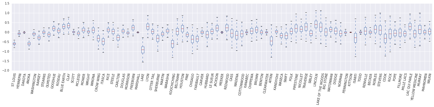
從這個盒鬚圖中,我們觀察到郡級別 \(\log(\text{UraniumPPM})\) 隨機效應的變異數隨著郡在資料集中表示的程度降低而增加。直覺上,這是有道理的,如果我們對某個郡的證據較少,我們應該對該郡的影響不太確定。
7 並排比較
我們現在比較所有三個程序的結果。為了做到這一點,我們將計算 Stan 和 TFP 產生的後驗樣本的非參數估計值。我們也將與 R 的 lme4 套件產生的參數(近似)估計值進行比較。
下圖描繪了明尼蘇達州每個郡的每個權重的後驗分配。我們顯示 Stan (紅色)、TFP (藍色) 和 R 的 lme4 (橙色) 的結果。我們為 Stan 和 TFP 的結果著色,因此預期在兩者一致時看到紫色。為了簡單起見,我們不為 R 的結果著色。每個子圖代表一個郡,並以光柵掃描順序(即從左到右,然後從上到下)依遞減頻率排序。
nrows = 17
ncols = 5
fig, ax = plt.subplots(nrows, ncols, figsize=(18, 21), sharey=True, sharex=True)
with warnings.catch_warnings():
  warnings.simplefilter('ignore')
  ii = -1
  for r in range(nrows):
    for c in range(ncols):
      ii += 1
      idx = county_freq[ii, 0]
      sns.kdeplot(
          posterior_random_weights_final_[:, idx] * log_county_uranium_ppm[idx],
          color='blue',
          alpha=.3,
          shade=True,
          label='TFP',
          ax=ax[r][c])
      sns.kdeplot(
          posterior_random_weights_final_stan[:, idx] *
          log_county_uranium_ppm[idx],
          color='red',
          alpha=.3,
          shade=True,
          label='Stan/rstanarm',
          ax=ax[r][c])
      sns.kdeplot(
          posterior_random_weights_lme4_final_[:, idx] *
          log_county_uranium_ppm[idx],
          color='#F4B400',
          alpha=.7,
          shade=False,
          label='R/lme4',
          ax=ax[r][c])
      ax[r][c].vlines(
          posterior_random_weights_lme4[idx] * log_county_uranium_ppm[idx],
          0,
          5,
          color='#F4B400',
          linestyle='--')
      ax[r][c].set_title(county_name[idx] + ' ({})'.format(idx), y=.7)
      ax[r][c].set_ylim(0, 5)
      ax[r][c].set_xlim(-1., 1.)
      ax[r][c].get_yaxis().set_visible(False)
      if ii == 2:
        ax[r][c].legend(bbox_to_anchor=(1.4, 1.7), fontsize=20, ncol=3)
      else:
        ax[r][c].legend_.remove()
  fig.subplots_adjust(wspace=0.03, hspace=0.1)
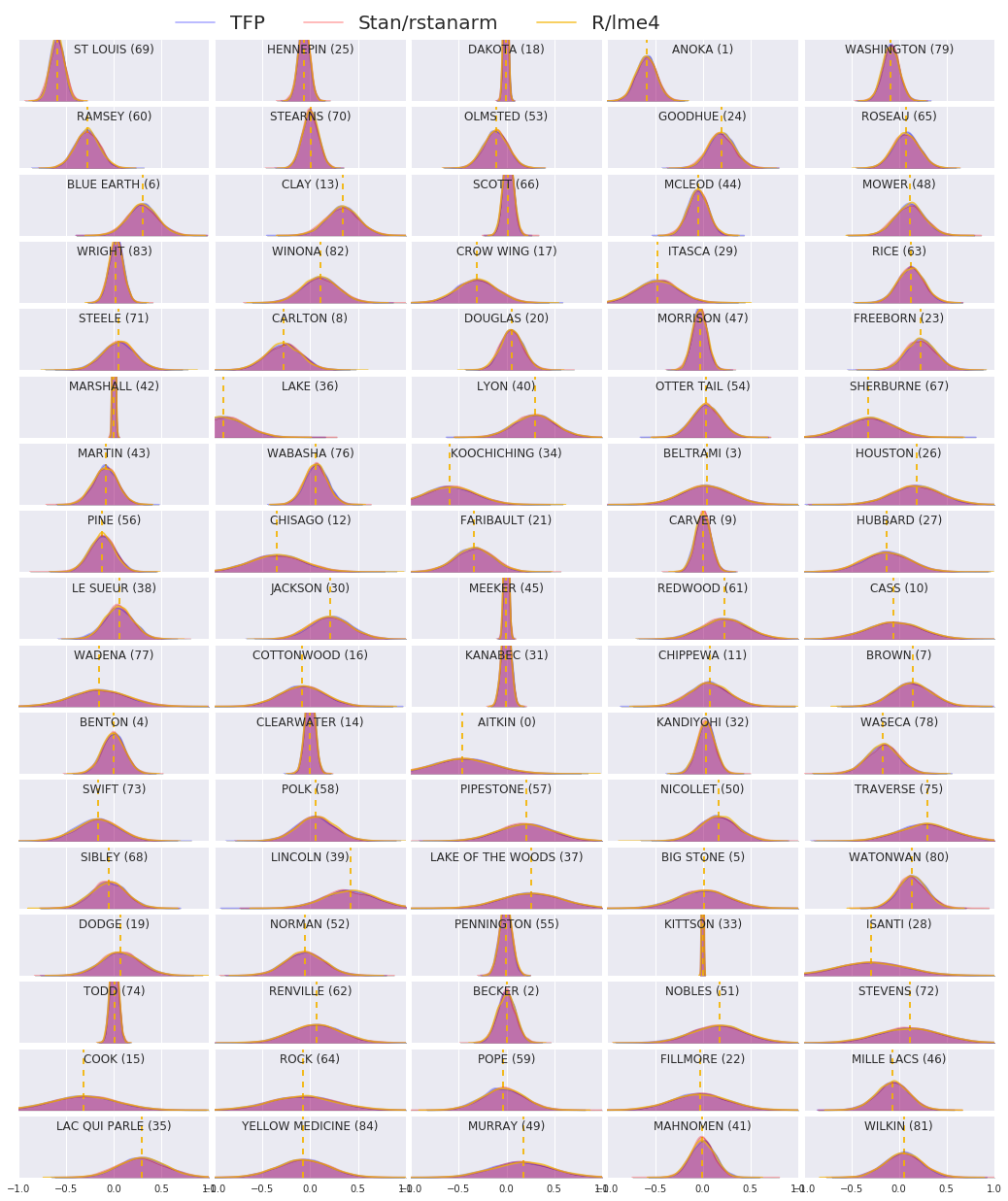
8 結論
在這個 Colab 中,我們將線性混合效應迴歸模型擬合到氡資料集。我們嘗試了三種不同的軟體套件:R、Stan 和 TensorFlow Probability。最後,我們繪製了由三種不同軟體套件計算出的 85 個後驗分配。
附錄 A:替代氡 HLM(新增隨機截距)
在本節中,我們描述了替代 HLM,它也具有與每個郡相關聯的隨機截距。
\[\begin{align*} \text{for } & c=1\ldots \text{NumCounties}:\\ & \beta_c \sim \text{MultivariateNormal}\left(\text{loc}=\left[ \begin{array}{c} 0 \\ 0 \end{array}\right] , \text{scale}=\left[\begin{array}{cc} \sigma_{11} & 0 \\ \sigma_{12} & \sigma_{22} \end{array}\right] \right) \\ \text{for } & i=1\ldots \text{NumSamples}:\\ & c_i := \text{County}_i \\ &\eta_i = \underbrace{\omega_0 + \omega_1\text{Floor}_i \vphantom{\log( \text{CountyUraniumPPM}_{c_i}))} }_{\text{固定效應} } + \underbrace{\beta_{c_i,0} + \beta_{c_i,1}\log( \text{CountyUraniumPPM}_{c_i}))}_{\text{隨機效應} } \\ &\log(\text{Radon}_i) \sim \text{Normal}(\text{loc}=\eta_i , \text{scale}=\sigma) \end{align*}\]
在 R 的 lme4「波浪符號表示法」中,此模型等效於
log_radon ~ 1 + floor + (1 + log_county_uranium_ppm | county)
附錄 B:廣義線性混合效應模型
在本節中,我們給出了比主體中使用的階層式線性模型更通用的特徵描述。這種更通用的模型稱為廣義線性混合效應模型 (GLMM)。
GLMM 是廣義線性模型 (GLM) 的推廣。GLMM 透過將樣本特定的隨機雜訊併入預測的線性回應中來擴充 GLM。這在一定程度上很有用,因為它允許很少見的功能與更常見的功能共用資訊。
作為生成過程,廣義線性混合效應模型 (GLMM) 的特徵是
\begin{align} \text{for } & r = 1\ldots R: \hspace{2.45cm}\text{# 針對每個隨機效應群組}\ &\begin{aligned} \text{for } &c = 1\ldots |Cr|: \hspace{1.3cm}\text{# 針對群組 \(r\) 的每個類別(「層級」)}\ &\begin{aligned} \beta{rc} &\sim \text{MultivariateNormal}(\text{loc}=0_{D_r}, \text{scale}=\Sigma_r^{1/2}) \end{aligned} \end{aligned}\\ \text{for } & i = 1 \ldots N: \hspace{2.45cm}\text{# 針對每個樣本}\ &\begin{aligned} &\etai = \underbrace{\vphantom{\sum{r=1}^R}xi^\top\omega}\text{固定效應} + \underbrace{\sum{r=1}^R z{r,i}^\top \beta_{r,Cr(i) } }\text{隨機效應} \ &Y_i|xi,\omega,{z{r,i} , \betar}{r=1}^R \sim \text{Distribution}(\text{mean}= g^{-1}(\eta_i)) \end{aligned} \end{align}
其中
\begin{align} R &= \text{隨機效應群組數量}\ |C_r| &= \text{群組 \(r\) 的類別數量}\ N &= \text{訓練樣本數量}\ x_i,\omega &\in \mathbb{R}^{D_0}\ D_0 &= \text{固定效應數量}\ Cr(i) &= \text{第 \(i\) 個樣本的類別(在群組 \(r\) 下)}\ z{r,i} &\in \mathbb{R}^{D_r}\ Dr &= \text{與群組 \(r\) 關聯的隨機效應數量}\ \Sigma{r} &\in {S\in\mathbb{R}^{D_r \times D_r} : S \succ 0 }\ \eta_i\mapsto g^{-1}(\eta_i) &= \mu_i, \text{反向連結函式}\ \text{Distribution} &=\text{僅可透過其平均數參數化的某些分配} \end{align}
用文字來說,這表示每個群組的每個類別都與 iid MVN \(\beta_{rc}\) 相關聯。雖然 \(\beta_{rc}\) 繪圖始終是獨立的,但它們僅針對群組 \(r\) 進行相同分配;請注意,每個 \(r\in\{1,\ldots,R\}\) 只有一個 \(\Sigma_r\)。
當與樣本群組的特徵 \(z_{r,i}\) 仿射組合時,結果是第 \(i\) 個預測線性回應(否則為 \(x_i^\top\omega\))上的樣本特定雜訊。
當我們估計 \(\{\Sigma_r:r\in\{1,\ldots,R\}\}\) 時,我們基本上是在估計隨機效應群組攜帶的雜訊量,否則會淹沒 \(x_i^\top\omega\) 中存在的訊號。
\(\text{Distribution}\) 和 反向連結函式 \(g^{-1}\) 有多種選項。常見的選擇是
- \(Y_i\sim\text{Normal}(\text{mean}=\eta_i, \text{scale}=\sigma)\),
- \(Y_i\sim\text{Binomial}(\text{mean}=n_i \cdot \text{sigmoid}(\eta_i), \text{total_count}=n_i)\),以及
- \(Y_i\sim\text{Poisson}(\text{mean}=\exp(\eta_i))\)。
如需更多可能性,請參閱 tfp.glm 模組。