
|
|
|
 在 GitHub 上檢視來源 在 GitHub 上檢視來源
|
|
在這個 Colab 中,我們將探索使用 TensorFlow 和 TensorFlow Probability 進行高斯過程迴歸。我們會從一些已知函數產生一些雜訊觀測值,並將 GP 模型擬合到這些資料。然後,我們會從 GP 後驗分佈中取樣,並在網格上繪製其定義域中取樣的函數值。
背景
令 \(\mathcal{X}\) 為任意集合。高斯過程 (GP) 是由 \(\mathcal{X}\) 索引的隨機變數集合,使得如果 \(\{X_1, \ldots, X_n\} \subset \mathcal{X}\) 是任何有限子集,則邊際密度 \(p(X_1 = x_1, \ldots, X_n = x_n)\) 是多變數高斯分佈。任何高斯分佈都完全由其第一和第二中心矩 (平均值和共變異數) 指定,GP 也不例外。我們可以根據其平均值函數 \(\mu : \mathcal{X} \to \mathbb{R}\) 和共變異數函數 \(k : \mathcal{X} \times \mathcal{X} \to \mathbb{R}\) 完全指定 GP。GP 的大多數表達能力都封裝在共變異數函數的選擇中。由於各種原因,共變異數函數也稱為核函數。僅要求它是對稱且正定的 (請參閱 Rasmussen & Williams 第 4 章)。以下我們使用 ExponentiatedQuadratic 共變異數核。其形式為
\[ k(x, x') := \sigma^2 \exp \left( \frac{\|x - x'\|^2}{\lambda^2} \right) \]
其中 \(\sigma^2\) 稱為「振幅」,\(\lambda\) 稱為長度尺度。可以透過最大概似最佳化程序選取核參數。
GP 的完整樣本包含整個空間 \(\mathcal{X}\) 上的實值函數,並且在實務上難以實現;通常,人們會選擇一組點來觀測樣本,並在這些點繪製函數值。這是透過從適當的 (有限維度) 多變數高斯分佈中取樣來實現的。
請注意,根據上述定義,任何有限維度多變數高斯分佈也是高斯過程。通常,當人們提到 GP 時,隱含的索引集是某個 \(\mathbb{R}^n\),我們在此確實會做出此假設。
高斯過程在機器學習中的常見應用是高斯過程迴歸。其想法是,我們希望在給定函數在有限數量的點 \(\{x_1, \ldots x_N\}.\) 處的雜訊觀測值 \(\{y_1, \ldots, y_N\}\) 的情況下,估計未知函數。我們想像一個生成過程
\[ \begin{align} f \sim \: & \textsf{GaussianProcess}\left( \text{mean_fn}=\mu(x), \text{covariance_fn}=k(x, x')\right) \\ y_i \sim \: & \textsf{Normal}\left( \text{loc}=f(x_i), \text{scale}=\sigma\right), i = 1, \ldots, N \end{align} \]
如上所述,由於我們需要在無限數量的點上取得其值,因此取樣函數無法計算。相反地,人們會考慮從多變數高斯分佈中取得有限樣本。
\[ \begin{gather} \begin{bmatrix} f(x_1) \\ \vdots \\ f(x_N) \end{bmatrix} \sim \textsf{MultivariateNormal} \left( \: \text{loc}= \begin{bmatrix} \mu(x_1) \\ \vdots \\ \mu(x_N) \end{bmatrix} \:,\: \text{scale}= \begin{bmatrix} k(x_1, x_1) & \cdots & k(x_1, x_N) \\ \vdots & \ddots & \vdots \\ k(x_N, x_1) & \cdots & k(x_N, x_N) \\ \end{bmatrix}^{1/2} \: \right) \end{gather} \\ y_i \sim \textsf{Normal} \left( \text{loc}=f(x_i), \text{scale}=\sigma \right) \]
請注意共變異數矩陣上的指數 \(\frac{1}{2}\):這表示 Cholesky 分解。計算 Cholesky 是必要的,因為 MVN 是位置-尺度族分佈。遺憾的是,Cholesky 分解的計算成本很高,需要 \(O(N^3)\) 時間和 \(O(N^2)\) 空間。GP 文獻的大部分內容都集中在處理這個看似無害的小指數。
通常將先驗平均值函數設為常數,通常為零。此外,某些符號慣例很方便。人們經常將 \(\mathbf{f}\) 寫為取樣函數值的有限向量。許多有趣的符號用於將 \(k\) 應用於輸入對而產生的共變異數矩陣。根據 (Quiñonero-Candela, 2005),我們注意到矩陣的組成部分是特定輸入點處函數值的共變異數。因此,我們可以將共變異數矩陣表示為 \(K_{AB}\),其中 \(A\) 和 \(B\) 是沿給定矩陣維度的函數值集合的一些指標。
例如,給定觀測資料 \((\mathbf{x}, \mathbf{y})\) 以及隱含的潛在函數值 \(\mathbf{f}\),我們可以寫成
\[ K_{\mathbf{f},\mathbf{f} } = \begin{bmatrix} k(x_1, x_1) & \cdots & k(x_1, x_N) \\ \vdots & \ddots & \vdots \\ k(x_N, x_1) & \cdots & k(x_N, x_N) \\ \end{bmatrix} \]
同樣地,我們可以混合輸入集,如
\[ K_{\mathbf{f},*} = \begin{bmatrix} k(x_1, x^*_1) & \cdots & k(x_1, x^*_T) \\ \vdots & \ddots & \vdots \\ k(x_N, x^*_1) & \cdots & k(x_N, x^*_T) \\ \end{bmatrix} \]
其中我們假設有 \(N\) 個訓練輸入和 \(T\) 個測試輸入。然後,上述生成過程可以簡潔地寫成
\[ \begin{align} \mathbf{f} \sim \: & \textsf{MultivariateNormal} \left( \text{loc}=\mathbf{0}, \text{scale}=K_{\mathbf{f},\mathbf{f} }^{1/2} \right) \\ y_i \sim \: & \textsf{Normal} \left( \text{loc}=f_i, \text{scale}=\sigma \right), i = 1, \ldots, N \end{align} \]
第一行中的取樣運算會從多變數高斯分佈產生一組有限的 \(N\) 個函數值,而不是如上述 GP 繪製符號中的整個函數。第二行描述了從以各種函數值為中心的單變數高斯分佈中取得的一組 \(N\) 個繪圖,並具有固定的觀測雜訊 \(\sigma^2\)。
有了上述生成模型,我們可以繼續考慮後驗推論問題。這會產生一組新的測試點處函數值的後驗分佈,以流程中上述觀察到的雜訊資料為條件。
有了上述符號,我們可以簡潔地寫出未來 (雜訊) 觀測值的後驗預測分佈,以對應的輸入和訓練資料為條件,如下所示 (如需更多詳細資訊,請參閱 Rasmussen & Williams 第 2.2 節)。
\[ \mathbf{y}^* \mid \mathbf{x}^*, \mathbf{x}, \mathbf{y} \sim \textsf{Normal} \left( \text{loc}=\mathbf{\mu}^*, \text{scale}=(\Sigma^*)^{1/2} \right), \]
其中
\[ \mathbf{\mu}^* = K_{*,\mathbf{f} }\left(K_{\mathbf{f},\mathbf{f} } + \sigma^2 I \right)^{-1} \mathbf{y} \]
且
\[ \Sigma^* = K_{*,*} - K_{*,\mathbf{f} } \left(K_{\mathbf{f},\mathbf{f} } + \sigma^2 I \right)^{-1} K_{\mathbf{f},*} \]
匯入
import time

import numpy as np
import matplotlib.pyplot as plt
import tensorflow as tf
import tf_keras
import tensorflow_probability as tfp
tfb = tfp.bijectors
tfd = tfp.distributions
tfk = tfp.math.psd_kernels

from mpl_toolkits.mplot3d import Axes3D
%pylab inline
# Configure plot defaults
plt.rcParams['axes.facecolor'] = 'white'
plt.rcParams['grid.color'] = '#666666'
%config InlineBackend.figure_format = 'png'
Populating the interactive namespace from numpy and matplotlib
範例:雜訊正弦波資料的精確 GP 迴歸
在這裡,我們會從雜訊正弦波產生訓練資料,然後從 GP 迴歸模型的後驗分佈中取樣一堆曲線。我們使用 Adam 來最佳化核超參數 (我們將先驗分佈下資料的負對數概似降至最低)。我們會繪製訓練曲線,然後繪製真實函數和後驗樣本。
def sinusoid(x):
  return np.sin(3 * np.pi * x[..., 0])

def generate_1d_data(num_training_points, observation_noise_variance):
  """Generate noisy sinusoidal observations at a random set of points.

  Returns:
     observation_index_points, observations
  """
  index_points_ = np.random.uniform(-1., 1., (num_training_points, 1))
  index_points_ = index_points_.astype(np.float64)
  # y = f(x) + noise
  observations_ = (sinusoid(index_points_) +
                   np.random.normal(loc=0,
                                    scale=np.sqrt(observation_noise_variance),
                                    size=(num_training_points)))
  return index_points_, observations_
# Generate training data with a known noise level (we'll later try to recover
# this value from the data).
NUM_TRAINING_POINTS = 100
observation_index_points_, observations_ = generate_1d_data(
    num_training_points=NUM_TRAINING_POINTS,
    observation_noise_variance=.1)
我們會在核超參數上放置先驗分佈,並使用 tfd.JointDistributionNamed 寫入超參數和觀測資料的聯合分佈。
def build_gp(amplitude, length_scale, observation_noise_variance):
  """Defines the conditional dist. of GP outputs, given kernel parameters."""

  # Create the covariance kernel, which will be shared between the prior (which we
  # use for maximum likelihood training) and the posterior (which we use for
  # posterior predictive sampling)
  kernel = tfk.ExponentiatedQuadratic(amplitude, length_scale)

  # Create the GP prior distribution, which we will use to train the model
  # parameters.
  return tfd.GaussianProcess(
      kernel=kernel,
      index_points=observation_index_points_,
      observation_noise_variance=observation_noise_variance)

gp_joint_model = tfd.JointDistributionNamed({
    'amplitude': tfd.LogNormal(loc=0., scale=np.float64(1.)),
    'length_scale': tfd.LogNormal(loc=0., scale=np.float64(1.)),
    'observation_noise_variance': tfd.LogNormal(loc=0., scale=np.float64(1.)),
    'observations': build_gp,
})
我們可以透過驗證是否可以從先驗分佈中取樣,以及計算樣本的對數密度,來進行實作的健全性檢查。
x = gp_joint_model.sample()
lp = gp_joint_model.log_prob(x)

print("sampled {}".format(x))
print("log_prob of sample: {}".format(lp))
sampled {'observation_noise_variance': <tf.Tensor: shape=(), dtype=float64, numpy=2.067952217184325>, 'length_scale': <tf.Tensor: shape=(), dtype=float64, numpy=1.154435715487831>, 'amplitude': <tf.Tensor: shape=(), dtype=float64, numpy=5.383850737703549>, 'observations': <tf.Tensor: shape=(100,), dtype=float64, numpy=
array([-2.37070577, -2.05363838, -0.95152824,  3.73509388, -0.2912646 ,
        0.46112342, -1.98018513, -2.10295857, -1.33589756, -2.23027226,
       -2.25081374, -0.89450835, -2.54196452,  1.46621647,  2.32016193,
        5.82399989,  2.27241034, -0.67523432, -1.89150197, -1.39834474,
       -2.33954116,  0.7785609 , -1.42763627, -0.57389025, -0.18226098,
       -3.45098732,  0.27986652, -3.64532398, -1.28635204, -2.42362875,
        0.01107288, -2.53222176, -2.0886136 , -5.54047694, -2.18389607,
       -1.11665628, -3.07161217, -2.06070336, -0.84464262,  1.29238438,
       -0.64973999, -2.63805504, -3.93317576,  0.65546645,  2.24721181,
       -0.73403676,  5.31628298, -1.2208384 ,  4.77782252, -1.42978168,
       -3.3089274 ,  3.25370494,  3.02117591, -1.54862932, -1.07360811,
        1.2004856 , -4.3017773 , -4.95787789, -1.95245901, -2.15960839,
       -3.78592731, -1.74096185,  3.54891595,  0.56294143,  1.15288455,
       -0.77323696,  2.34430694, -1.05302007, -0.7514684 , -0.98321063,
       -3.01300144, -3.00033274,  0.44200837,  0.45060886, -1.84497318,
       -1.89616746, -2.15647664, -2.65672581, -3.65493379,  1.70923375,
       -3.88695218, -0.05151283,  4.51906677, -2.28117003,  3.03032793,
       -1.47713194, -0.35625273,  3.73501587, -2.09328047, -0.60665614,
       -0.78177188, -0.67298545,  2.97436033, -0.29407932,  2.98482427,
       -1.54951178,  2.79206821,  4.2225733 ,  2.56265198,  2.80373284])>}
log_prob of sample: -194.96442183797524
現在讓我們最佳化以找出具有最高後驗機率的參數值。我們會為每個參數定義一個變數,並限制其值為正數。
# Create the trainable model parameters, which we'll subsequently optimize.
# Note that we constrain them to be strictly positive.

constrain_positive = tfb.Shift(np.finfo(np.float64).tiny)(tfb.Exp())

amplitude_var = tfp.util.TransformedVariable(
    initial_value=1.,
    bijector=constrain_positive,
    name='amplitude',
    dtype=np.float64)

length_scale_var = tfp.util.TransformedVariable(
    initial_value=1.,
    bijector=constrain_positive,
    name='length_scale',
    dtype=np.float64)

observation_noise_variance_var = tfp.util.TransformedVariable(
    initial_value=1.,
    bijector=constrain_positive,
    name='observation_noise_variance_var',
    dtype=np.float64)

trainable_variables = [v.trainable_variables[0] for v in
                       [amplitude_var,
                       length_scale_var,
                       observation_noise_variance_var]]
為了以我們的觀測資料為條件設定模型,我們會定義一個 target_log_prob 函數,該函數會採用 (仍待推斷的) 核超參數。
def target_log_prob(amplitude, length_scale, observation_noise_variance):
  return gp_joint_model.log_prob({
      'amplitude': amplitude,
      'length_scale': length_scale,
      'observation_noise_variance': observation_noise_variance,
      'observations': observations_
  })
# Now we optimize the model parameters.
num_iters = 1000
optimizer = tf_keras.optimizers.Adam(learning_rate=.01)

# Use `tf.function` to trace the loss for more efficient evaluation.
@tf.function(autograph=False, jit_compile=False)
def train_model():
  with tf.GradientTape() as tape:
    loss = -target_log_prob(amplitude_var, length_scale_var,
                            observation_noise_variance_var)
  grads = tape.gradient(loss, trainable_variables)
  optimizer.apply_gradients(zip(grads, trainable_variables))
  return loss

# Store the likelihood values during training, so we can plot the progress
lls_ = np.zeros(num_iters, np.float64)
for i in range(num_iters):
  loss = train_model()
  lls_[i] = loss

print('Trained parameters:')
print('amplitude: {}'.format(amplitude_var._value().numpy()))
print('length_scale: {}'.format(length_scale_var._value().numpy()))
print('observation_noise_variance: {}'.format(observation_noise_variance_var._value().numpy()))
Trained parameters:
amplitude: 0.9176153445125278
length_scale: 0.18444082442910079
observation_noise_variance: 0.0880273312850989
# Plot the loss evolution
plt.figure(figsize=(12, 4))
plt.plot(lls_)
plt.xlabel("Training iteration")
plt.ylabel("Log marginal likelihood")
plt.show()

# Having trained the model, we'd like to sample from the posterior conditioned
# on observations. We'd like the samples to be at points other than the training
# inputs.
predictive_index_points_ = np.linspace(-1.2, 1.2, 200, dtype=np.float64)
# Reshape to [200, 1] -- 1 is the dimensionality of the feature space.
predictive_index_points_ = predictive_index_points_[..., np.newaxis]

optimized_kernel = tfk.ExponentiatedQuadratic(amplitude_var, length_scale_var)
gprm = tfd.GaussianProcessRegressionModel(
    kernel=optimized_kernel,
    index_points=predictive_index_points_,
    observation_index_points=observation_index_points_,
    observations=observations_,
    observation_noise_variance=observation_noise_variance_var,
    predictive_noise_variance=0.)

# Create op to draw  50 independent samples, each of which is a *joint* draw
# from the posterior at the predictive_index_points_. Since we have 200 input
# locations as defined above, this posterior distribution over corresponding
# function values is a 200-dimensional multivariate Gaussian distribution!
num_samples = 50
samples = gprm.sample(num_samples)
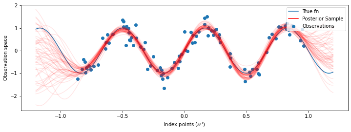
# Plot the true function, observations, and posterior samples.
plt.figure(figsize=(12, 4))
plt.plot(predictive_index_points_, sinusoid(predictive_index_points_),
         label='True fn')
plt.scatter(observation_index_points_[:, 0], observations_,
            label='Observations')
for i in range(num_samples):
  plt.plot(predictive_index_points_, samples[i, :], c='r', alpha=.1,
           label='Posterior Sample' if i == 0 else None)
leg = plt.legend(loc='upper right')
for lh in leg.legendHandles:
    lh.set_alpha(1)
plt.xlabel(r"Index points ($\mathbb{R}^1$)")
plt.ylabel("Observation space")
plt.show()
使用 HMC 邊緣化超參數
讓我們嘗試使用 Hamiltonian Monte Carlo 來積分出超參數,而不是最佳化超參數。我們會先定義並執行取樣器,以大約從給定觀測值的核超參數後驗分佈中繪製樣本。
num_results = 100
num_burnin_steps = 50

sampler = tfp.mcmc.TransformedTransitionKernel(
    tfp.mcmc.NoUTurnSampler(
        target_log_prob_fn=target_log_prob,
        step_size=tf.cast(0.1, tf.float64)),
    bijector=[constrain_positive, constrain_positive, constrain_positive])

adaptive_sampler = tfp.mcmc.DualAveragingStepSizeAdaptation(
    inner_kernel=sampler,
    num_adaptation_steps=int(0.8 * num_burnin_steps),
    target_accept_prob=tf.cast(0.75, tf.float64))

initial_state = [tf.cast(x, tf.float64) for x in [1., 1., 1.]]
# Speed up sampling by tracing with `tf.function`.
@tf.function(autograph=False, jit_compile=False)
def do_sampling():
  return tfp.mcmc.sample_chain(
      kernel=adaptive_sampler,
      current_state=initial_state,
      num_results=num_results,
      num_burnin_steps=num_burnin_steps,
      trace_fn=lambda current_state, kernel_results: kernel_results)

t0 = time.time()
samples, kernel_results = do_sampling()
t1 = time.time()
print("Inference ran in {:.2f}s.".format(t1-t0))
Inference ran in 9.00s.
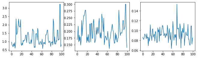
讓我們透過檢查超參數追蹤來進行取樣器的健全性檢查。
(amplitude_samples,
 length_scale_samples,
 observation_noise_variance_samples) = samples

f = plt.figure(figsize=[15, 3])
for i, s in enumerate(samples):
  ax = f.add_subplot(1, len(samples) + 1, i + 1)
  ax.plot(s)
現在,我們不是建構具有最佳化超參數的單個 GP,而是將後驗預測分佈建構為 GP 的混合,每個 GP 都由超參數後驗分佈中的樣本定義。這大約透過蒙地卡羅取樣來整合後驗參數,以計算未觀測位置的邊際預測分佈。
# The sampled hyperparams have a leading batch dimension, `[num_results, ...]`,
# so they construct a *batch* of kernels.
batch_of_posterior_kernels = tfk.ExponentiatedQuadratic(
    amplitude_samples, length_scale_samples)

# The batch of kernels creates a batch of GP predictive models, one for each
# posterior sample.
batch_gprm = tfd.GaussianProcessRegressionModel(
    kernel=batch_of_posterior_kernels,
    index_points=predictive_index_points_,
    observation_index_points=observation_index_points_,
    observations=observations_,
    observation_noise_variance=observation_noise_variance_samples,
    predictive_noise_variance=0.)

# To construct the marginal predictive distribution, we average with uniform
# weight over the posterior samples.
predictive_gprm = tfd.MixtureSameFamily(
    mixture_distribution=tfd.Categorical(logits=tf.zeros([num_results])),
    components_distribution=batch_gprm)

num_samples = 50
samples = predictive_gprm.sample(num_samples)
# Plot the true function, observations, and posterior samples.
plt.figure(figsize=(12, 4))
plt.plot(predictive_index_points_, sinusoid(predictive_index_points_),
         label='True fn')
plt.scatter(observation_index_points_[:, 0], observations_,
            label='Observations')
for i in range(num_samples):
  plt.plot(predictive_index_points_, samples[i, :], c='r', alpha=.1,
           label='Posterior Sample' if i == 0 else None)
leg = plt.legend(loc='upper right')
for lh in leg.legendHandles:
    lh.set_alpha(1)
plt.xlabel(r"Index points ($\mathbb{R}^1$)")
plt.ylabel("Observation space")
plt.show()
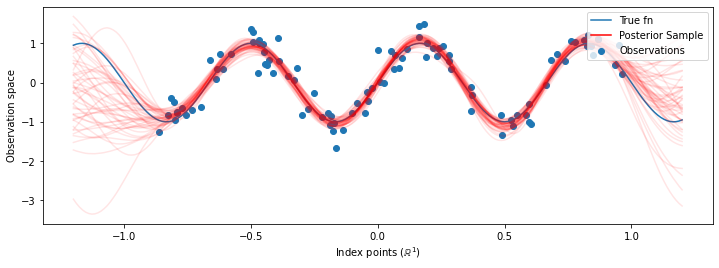
雖然在這種情況下差異很細微,但一般而言,我們預期後驗預測分佈比僅使用我們在上面執行的最可能參數更能更好地泛化 (為保留資料提供更高的概似)。