
|
|
|
 在 GitHub 上檢視原始碼 在 GitHub 上檢視原始碼
|
|
潛在變數模型試圖捕捉高維度資料中的隱藏結構。範例包括主成分分析 (PCA) 和因子分析。高斯過程是「非參數」模型,可以彈性地捕捉局部相關結構和不確定性。高斯過程潛在變數模型 (Lawrence, 2004) 結合了這些概念。
背景:高斯過程
高斯過程是隨機變數的任何集合,使得任何有限子集的邊際分佈都是多變量常態分佈。如需深入瞭解迴歸背景中的 GP,請查看 TensorFlow Probability 中的高斯過程迴歸。
我們使用所謂的索引集來標記 GP 所包含的集合中每個隨機變數。在有限索引集的情況下,我們只會得到一個多變量常態分佈。然而,當我們考慮無限集合時,GP 最有趣。在像 \(\mathbb{R}^D\) 這樣的索引集的情況下,其中我們在 \(D\) 維空間中的每個點都有一個隨機變數,GP 可以被認為是隨機函數的分佈。如果可以實現,從這樣的 GP 中單次提取將為 \(\mathbb{R}^D\) 中的每個點分配一個(聯合常態分佈)值。在本 Colab 中,我們將重點關注某些 \(\mathbb{R}^D\) 上的 GP。
常態分佈完全由其一階和二階統計量決定——實際上,定義常態分佈的一種方法是將其定義為高階累積量均為零的分佈。GP 也是如此:我們透過描述均值和共變異數* 來完全指定 GP。回想一下,對於有限維多變量常態分佈,均值是一個向量,而共變異數是一個方形、對稱正定矩陣。在無限維 GP 中,這些結構推廣到均值函數 \(m : \mathbb{R}^D \to \mathbb{R}\)(在索引集的每個點定義)和共變異數「核心」函數 \(k : \mathbb{R}^D \times \mathbb{R}^D \to \mathbb{R}\)。核心函數必須是正定的,這基本上表示,限制在有限點集時,它會產生一個正定矩陣。
GP 的大部分結構都源自其共變異數核心函數——此函數描述了採樣函數的值如何在附近(或不太附近的)點之間變化。不同的共變異數函數鼓勵不同的平滑度。一種常用的核心函數是「指數二次」(又稱「高斯」、「平方指數」或「徑向基底函數」),\(k(x, x') = \sigma^2 e^{(x - x^2) / \lambda^2}\)。其他範例在 David Duvenaud 的核心食譜頁面以及經典文本《Gaussian Processes for Machine Learning》中概述。
* 對於無限索引集,我們還需要一致性條件。由於 GP 的定義是根據有限邊際值,因此我們必須要求這些邊際值是一致的,而與邊際值的取得順序無關。這是隨機過程理論中一個有些進階的主題,超出本教學的範圍;可以說,最終一切都會順利解決!
應用 GP:迴歸和潛在變數模型
我們可以使用 GP 的一種方法是用於迴歸:給定以輸入 \(\{x_i\}_{i=1}^N\)(索引集的元素)和觀察值 \(\{y_i\}_{i=1}^N\) 形式的大量觀察資料,我們可以使用這些資料在新點集 \(\{x_j^*\}_{j=1}^M\) 處形成後驗預測分佈。由於分佈都是高斯分佈,這歸結為一些簡單的線性代數(但請注意:必要的計算的執行時間與資料點的數量成三次關係,並且所需的空間與資料點的數量成二次關係——這是 GP 使用中的主要限制因素,目前許多研究都集中在精確後驗推論的計算上可行的替代方案)。我們在 TFP Colab 中的 GP 迴歸中更詳細地介紹了 GP 迴歸。
我們可以使用 GP 的另一種方法是作為潛在變數模型:給定高維度觀察值(例如,圖像)的集合,我們可以假設一些低維度潛在結構。我們假設,以潛在結構為條件,大量輸出(圖像中的像素)彼此獨立。此模型中的訓練包括
- 最佳化模型參數(核心函數參數以及例如觀察雜訊變異數),以及
- 針對每個訓練觀察值(圖像),在索引集中找到對應的點位置。所有最佳化都可以透過最大化資料的邊際對數似然性來完成。
匯入
import numpy as np
import tensorflow as tf
import tf_keras
import tensorflow_probability as tfp
tfd = tfp.distributions
tfk = tfp.math.psd_kernels
%pylab inline
Populating the interactive namespace from numpy and matplotlib
載入 MNIST 資料
# Load the MNIST data set and isolate a subset of it.
(x_train, y_train), (_, _) = tf_keras.datasets.mnist.load_data()
N = 1000
small_x_train = x_train[:N, ...].astype(np.float64) / 256.
small_y_train = y_train[:N]
Downloading data from https://storage.googleapis.com/tensorflow/tf-keras-datasets/mnist.npz
11493376/11490434 [==============================] - 0s 0us/step
11501568/11490434 [==============================] - 0s 0us/step
準備可訓練變數
我們將聯合訓練 3 個模型參數以及潛在輸入。
# Create some trainable model parameters. We will constrain them to be strictly
# positive when constructing the kernel and the GP.
unconstrained_amplitude = tf.Variable(np.float64(1.), name='amplitude')
unconstrained_length_scale = tf.Variable(np.float64(1.), name='length_scale')
unconstrained_observation_noise = tf.Variable(np.float64(1.), name='observation_noise')
# We need to flatten the images and, somewhat unintuitively, transpose from
# shape [100, 784] to [784, 100]. This is because the 784 pixels will be
# treated as *independent* conditioned on the latent inputs, meaning we really
# have a batch of 784 GP's with 100 index_points.
observations_ = small_x_train.reshape(N, -1).transpose()

# Create a collection of N 2-dimensional index points that will represent our
# latent embeddings of the data. (Lawrence, 2004) prescribes initializing these
# with PCA, but a random initialization actually gives not-too-bad results, so
# we use this for simplicity. For a fun exercise, try doing the
# PCA-initialization yourself!
init_ = np.random.normal(size=(N, 2))
latent_index_points = tf.Variable(init_, name='latent_index_points')
建構模型和訓練運算
# Create our kernel and GP distribution
EPS = np.finfo(np.float64).eps

def create_kernel():
  amplitude = tf.math.softplus(EPS + unconstrained_amplitude)
  length_scale = tf.math.softplus(EPS + unconstrained_length_scale)
  kernel = tfk.ExponentiatedQuadratic(amplitude, length_scale)
  return kernel

def loss_fn():
  observation_noise_variance = tf.math.softplus(
      EPS + unconstrained_observation_noise)
  gp = tfd.GaussianProcess(
      kernel=create_kernel(),
      index_points=latent_index_points,
      observation_noise_variance=observation_noise_variance)
  log_probs = gp.log_prob(observations_, name='log_prob')
  return -tf.reduce_mean(log_probs)

trainable_variables = [unconstrained_amplitude,
                       unconstrained_length_scale,
                       unconstrained_observation_noise,
                       latent_index_points]

optimizer = tf_keras.optimizers.Adam(learning_rate=1.0)

@tf.function(autograph=False, jit_compile=True)
def train_model():
  with tf.GradientTape() as tape:
    loss_value = loss_fn()
  grads = tape.gradient(loss_value, trainable_variables)
  optimizer.apply_gradients(zip(grads, trainable_variables))
  return loss_value
訓練並繪製產生的潛在嵌入
# Initialize variables and train!
num_iters = 100
log_interval = 20
lips = np.zeros((num_iters, N, 2), np.float64)
for i in range(num_iters):
  loss = train_model()
  lips[i] = latent_index_points.numpy()
  if i % log_interval == 0 or i + 1 == num_iters:
    print("Loss at step %d: %f" % (i, loss))
Loss at step 0: 1108.121688
Loss at step 20: -159.633761
Loss at step 40: -263.014394
Loss at step 60: -283.713056
Loss at step 80: -288.709413
Loss at step 99: -289.662253
繪製結果
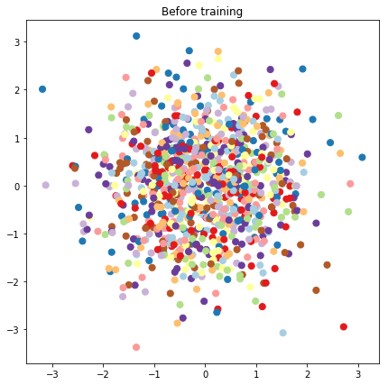
# Plot the latent locations before and after training
plt.figure(figsize=(7, 7))
plt.title("Before training")
plt.grid(False)
plt.scatter(x=init_[:, 0], y=init_[:, 1],
c=y_train[:N], cmap=plt.get_cmap('Paired'), s=50)
plt.show()
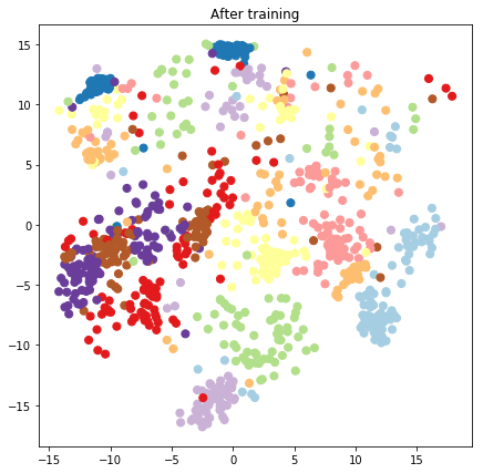
plt.figure(figsize=(7, 7))
plt.title("After training")
plt.grid(False)
plt.scatter(x=lips[-1, :, 0], y=lips[-1, :, 1],
c=y_train[:N], cmap=plt.get_cmap('Paired'), s=50)
plt.show()
建構預測模型和採樣運算
# We'll draw samples at evenly spaced points on a 10x10 grid in the latent
# input space.
sample_grid_points = 10
grid_ = np.linspace(-4, 4, sample_grid_points).astype(np.float64)
# Create a 10x10 grid of 2-vectors, for a total shape [10, 10, 2]
grid_ = np.stack(np.meshgrid(grid_, grid_), axis=-1)

# This part's a bit subtle! What we defined above was a batch of 784 (=28x28)
# independent GP distributions over the input space. Each one corresponds to a
# single pixel of an MNIST image. Now what we'd like to do is draw 100 (=10x10)
# *independent* samples, each one separately conditioned on all the observations
# as well as the learned latent input locations above.
#
# The GP regression model below will define a batch of 784 independent
# posteriors. We'd like to get 100 independent samples each at a different
# latent index point. We could loop over the points in the grid, but that might
# be a bit slow. Instead, we can vectorize the computation by tacking on *even
# more* batch dimensions to our GaussianProcessRegressionModel distribution.
# In the below grid_ shape, we have concatentaed
#   1. batch shape: [sample_grid_points, sample_grid_points, 1]
#   2. number of examples: [1]
#   3. number of latent input dimensions: [2]
# The `1` in the batch shape will broadcast with 784. The final result will be
# samples of shape [10, 10, 784, 1]. The `1` comes from the "number of examples"
# and we can just `np.squeeze` it off.
grid_ = grid_.reshape(sample_grid_points, sample_grid_points, 1, 1, 2)

# Create the GPRegressionModel instance which represents the posterior
# predictive at the grid of new points.
gprm = tfd.GaussianProcessRegressionModel(
    kernel=create_kernel(),
    # Shape [10, 10, 1, 1, 2]
    index_points=grid_,
    # Shape [1000, 2]. 1000 2 dimensional vectors.
    observation_index_points=latent_index_points,
    # Shape [784, 1000]. A batch of 784 1000-dimensional observations.
    observations=observations_)
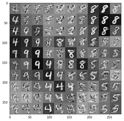
繪製以資料和潛在嵌入為條件的樣本
我們在潛在空間中的 2 維網格上的 100 個點進行採樣。
samples = gprm.sample()

# Plot the grid of samples at new points. We do a bit of tweaking of the samples
# first, squeezing off extra 1-shapes and normalizing the values.
samples_ = np.squeeze(samples.numpy())
samples_ = ((samples_ -
             samples_.min(-1, keepdims=True)) /
            (samples_.max(-1, keepdims=True) -
             samples_.min(-1, keepdims=True)))
samples_ = samples_.reshape(sample_grid_points, sample_grid_points, 28, 28)
samples_ = samples_.transpose([0, 2, 1, 3])
samples_ = samples_.reshape(28 * sample_grid_points, 28 * sample_grid_points)
plt.figure(figsize=(7, 7))
ax = plt.subplot()
ax.grid(False)
ax.imshow(-samples_, interpolation='none', cmap='Greys')
plt.show()
結論
我們簡要介紹了高斯過程潛在變數模型,並展示瞭如何僅用幾行 TF 和 TF Probability 程式碼來實作它。