在 TensorFlow.org 上檢視

在 Google Colab 中執行

在 GitHub 上檢視原始碼

下載筆記本

import numpy as np
import matplotlib.pyplot as plt
import tensorflow.compat.v2 as tf
tf.enable_v2_behavior()

import tensorflow_probability as tfp
tfd = tfp.distributions
tfb = tfp.bijectors

「[copula](https://en.wikipedia.org/wiki/Copula_(probability_theory%29) 」是一種用於擷取隨機變數之間依賴關係的古典方法。更正式地說，copula 是一種多變數分配 \(C(U_1, U_2, ...., U_n)\)，因此邊緣化會產生 \(U_i \sim \text{Uniform}(0, 1)\) 的結果。

Copula 很有趣，因為我們可以使用它們建立具有任意邊際的多變數分配。以下是方法

• 使用「機率積分轉換」會將任意連續隨機變數 \(X\) 轉換為均勻隨機變數 \(F_X(X)\)，其中 \(F_X\) 是 \(X\) 的 CDF。
• 假設給定 copula (例如雙變數) \(C(U, V)\)，我們知道 \(U\) 和 \(V\) 具有均勻邊際分配。
• 現在假設給定我們感興趣的隨機變數 \(X, Y\)，建立新的分配 \(C'(X, Y) = C(F_X(X), F_Y(Y))\)。\(X\) 和 \(Y\) 的邊際是我們想要的。

邊際是單變數的，因此可能更容易測量和/或建模。Copula 能夠從邊際開始，同時也能在維度之間實現任意相關性。

高斯 Copula

為了說明如何建構 copula，請考量根據多變數高斯相關性擷取依賴關係的情況。高斯 Copula 是由 \(C(u_1, u_2, ...u_n) = \Phi_\Sigma(\Phi^{-1}(u_1), \Phi^{-1}(u_2), ... \Phi^{-1}(u_n))\) 給定的 copula，其中 \(\Phi_\Sigma\) 代表 MultivariateNormal 的 CDF，共變異數為 \(\Sigma\) 且平均值為 0，而 \(\Phi^{-1}\) 是標準常態的反向 CDF。

套用常態的反向 CDF 會扭曲均勻維度，使其呈常態分配。然後套用多變數常態的 CDF 會擠壓分配，使其在邊際上均勻，並具有高斯相關性。

因此，我們得到的是高斯 Copula 是一種在單位超立方體 \([0, 1]^n\) 上具有均勻邊際的分配。

如此定義後，可以使用 tfd.TransformedDistribution 和適當的 Bijector 實作高斯 Copula。也就是說，我們正在轉換 MultivariateNormal，方法是使用常態分配的反向 CDF，此 CDF 由 tfb.NormalCDF 雙射器實作。

在下方，我們使用一個簡化假設實作高斯 Copula：共變異數由 Cholesky 因子參數化 (因此是 MultivariateNormalTriL 的共變異數)。(可以使用其他 tf.linalg.LinearOperators 來編碼不同的無矩陣假設。)。

class GaussianCopulaTriL(tfd.TransformedDistribution):
  """Takes a location, and lower triangular matrix for the Cholesky factor."""
  def __init__(self, loc, scale_tril):
    super(GaussianCopulaTriL, self).__init__(
        distribution=tfd.MultivariateNormalTriL(
            loc=loc,
            scale_tril=scale_tril),
        bijector=tfb.NormalCDF(),
        validate_args=False,
        name="GaussianCopulaTriLUniform")


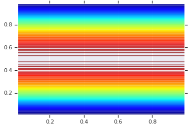
# Plot an example of this.
unit_interval = np.linspace(0.01, 0.99, num=200, dtype=np.float32)
x_grid, y_grid = np.meshgrid(unit_interval, unit_interval)
coordinates = np.concatenate(
    [x_grid[..., np.newaxis],
     y_grid[..., np.newaxis]], axis=-1)

pdf = GaussianCopulaTriL(
    loc=[0., 0.],
    scale_tril=[[1., 0.8], [0., 0.6]],
).prob(coordinates)

# Plot its density.

plt.contour(x_grid, y_grid, pdf, 100, cmap=plt.cm.jet);

然而，此類模型的威力在於使用機率積分轉換，以在任意隨機變數上使用 copula。透過這種方式，我們可以指定任意邊際，並使用 copula 將它們縫合在一起。

我們先從模型開始

\[\begin{align*} X &\sim \text{Kumaraswamy}(a, b) \\ Y &\sim \text{Gumbel}(\mu, \beta) \end{align*}\]

並使用 copula 取得雙變數隨機變數 \(Z\)，其具有 Kumaraswamy 和 Gumbel 邊際。

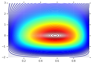
我們先繪製由這兩個隨機變數產生的乘積分配圖。這僅作為套用 Copula 時的比較點。

a = 2.0
b = 2.0
gloc = 0.
gscale = 1.

x = tfd.Kumaraswamy(a, b)
y = tfd.Gumbel(loc=gloc, scale=gscale)

# Plot the distributions, assuming independence
x_axis_interval = np.linspace(0.01, 0.99, num=200, dtype=np.float32)
y_axis_interval = np.linspace(-2., 3., num=200, dtype=np.float32)
x_grid, y_grid = np.meshgrid(x_axis_interval, y_axis_interval)

pdf = x.prob(x_grid) * y.prob(y_grid)

# Plot its density

plt.contour(x_grid, y_grid, pdf, 100, cmap=plt.cm.jet);

具有不同邊際的聯合分配

現在我們使用高斯 copula 將分配耦合在一起，並繪製圖表。同樣地，我們選擇的工具是 TransformedDistribution，套用適當的 Bijector 以取得選定的邊際。

具體來說，我們使用 Blockwise 雙射器，它在向量的不同部分套用不同的雙射器 (這仍然是雙射轉換)。

現在我們可以定義想要的 Copula。假設給定目標邊際清單 (編碼為雙射器)，我們可以輕鬆建構使用 copula 並具有指定邊際的新分配。

class WarpedGaussianCopula(tfd.TransformedDistribution):
  """Application of a Gaussian Copula on a list of target marginals.

  This implements an application of a Gaussian Copula. Given [x_0, ... x_n]
  which are distributed marginally (with CDF) [F_0, ... F_n],
  `GaussianCopula` represents an application of the Copula, such that the
  resulting multivariate distribution has the above specified marginals.

  The marginals are specified by `marginal_bijectors`: These are
  bijectors whose `inverse` encodes the CDF and `forward` the inverse CDF.

  block_sizes is a 1-D Tensor to determine splits for `marginal_bijectors`
  length should be same as length of `marginal_bijectors`.
  See tfb.Blockwise for details
  """
  def __init__(self, loc, scale_tril, marginal_bijectors, block_sizes=None):
    super(WarpedGaussianCopula, self).__init__(
        distribution=GaussianCopulaTriL(loc=loc, scale_tril=scale_tril),
        bijector=tfb.Blockwise(bijectors=marginal_bijectors,
                               block_sizes=block_sizes),
        validate_args=False,
        name="GaussianCopula")

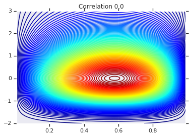
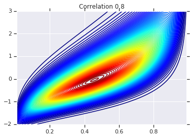
最後，讓我們實際使用此高斯 Copula。我們將使用 \(\begin{bmatrix}1 & 0\\\rho & \sqrt{(1-\rho^2)}\end{bmatrix}\) 的 Cholesky，它將對應於變異數 1，以及多變數常態的相關性 \(\rho\)。

我們將查看幾個案例

# Create our coordinates:
coordinates = np.concatenate(
    [x_grid[..., np.newaxis], y_grid[..., np.newaxis]], -1)


def create_gaussian_copula(correlation):
  # Use Gaussian Copula to add dependence.
  return WarpedGaussianCopula(
      loc=[0.,  0.],
      scale_tril=[[1., 0.], [correlation, tf.sqrt(1. - correlation ** 2)]],
      # These encode the marginals we want. In this case we want X_0 has
      # Kumaraswamy marginal, and X_1 has Gumbel marginal.

      marginal_bijectors=[
          tfb.Invert(tfb.KumaraswamyCDF(a, b)),
          tfb.Invert(tfb.GumbelCDF(loc=0., scale=1.))])


# Note that the zero case will correspond to independent marginals!
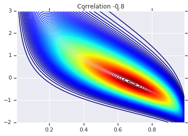
correlations = [0., -0.8, 0.8]
copulas = []
probs = []
for correlation in correlations:
  copula = create_gaussian_copula(correlation)
  copulas.append(copula)
  probs.append(copula.prob(coordinates))


# Plot it's density

for correlation, copula_prob in zip(correlations, probs):
  plt.figure()
  plt.contour(x_grid, y_grid, copula_prob, 100, cmap=plt.cm.jet)
  plt.title('Correlation {}'.format(correlation))

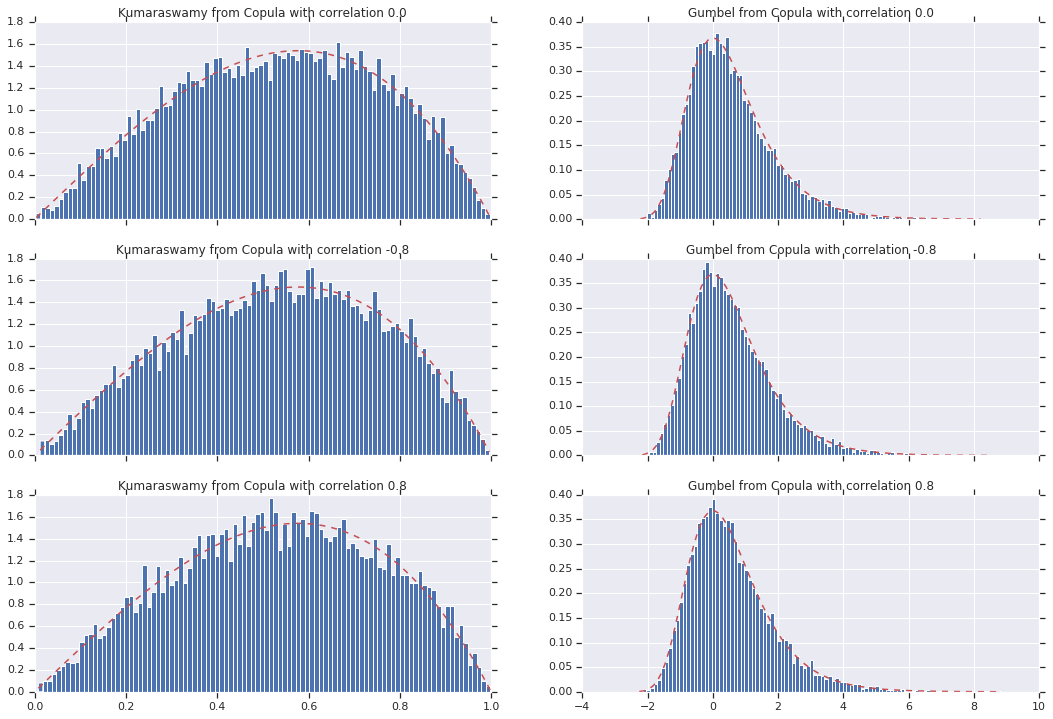
最後，讓我們驗證我們是否確實獲得了想要的邊際。

def kumaraswamy_pdf(x):
    return tfd.Kumaraswamy(a, b).prob(np.float32(x))

def gumbel_pdf(x):
    return tfd.Gumbel(gloc, gscale).prob(np.float32(x))


copula_samples = []
for copula in copulas:
  copula_samples.append(copula.sample(10000))

plot_rows = len(correlations)
plot_cols = 2  # for 2  densities [kumarswamy, gumbel]
fig, axes = plt.subplots(plot_rows, plot_cols, sharex='col', figsize=(18,12))

# Let's marginalize out on each, and plot the samples.

for i, (correlation, copula_sample) in enumerate(zip(correlations, copula_samples)):
  k = copula_sample[..., 0].numpy()
  g = copula_sample[..., 1].numpy()


  _, bins, _ = axes[i, 0].hist(k, bins=100, density=True)
  axes[i, 0].plot(bins, kumaraswamy_pdf(bins), 'r--')
  axes[i, 0].set_title('Kumaraswamy from Copula with correlation {}'.format(correlation))

  _, bins, _ = axes[i, 1].hist(g, bins=100, density=True)
  axes[i, 1].plot(bins, gumbel_pdf(bins), 'r--')
  axes[i, 1].set_title('Gumbel from Copula with correlation {}'.format(correlation))

結論

就這樣！我們已示範可以使用 Bijector API 建構高斯 Copula。

更一般來說，使用 Bijector API 撰寫雙射器，並將它們與分配組合，可以為彈性建模建立豐富的分配系列。