
|
|
|
 在 GitHub 上檢視原始碼 在 GitHub 上檢視原始碼
|
|
在這份筆記本中,我們將示範如何透過擬合高斯分佈的狄利克雷過程混合模型,對大量樣本進行分群,並同時推斷叢集數量。我們使用預處理隨機梯度朗之萬動力學 (pSGLD) 進行推論。
目錄
樣本
模型
最佳化
將結果視覺化
4.1. 分群結果
4.2. 將不確定性視覺化
4.3. 所選混合成分的平均值與尺度
4.4. 各混合成分的混合權重
4.5. \(\alpha\) 的收斂性
4.6. 迭代次數中的推論叢集數量
4.7. 使用 RMSProp 擬合模型
結論
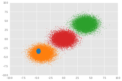
1. 樣本
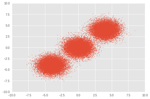
首先,我們設定一個玩具資料集。我們從三個雙變量高斯分佈中產生 50,000 個隨機樣本。
import time
import numpy as np
import matplotlib.pyplot as plt
import tensorflow.compat.v1 as tf
import tensorflow_probability as tfp
plt.style.use('ggplot')
tfd = tfp.distributions
def session_options(enable_gpu_ram_resizing=True):
  """Convenience function which sets common `tf.Session` options."""
  config = tf.ConfigProto()
  config.log_device_placement = True
  if enable_gpu_ram_resizing:
    # `allow_growth=True` makes it possible to connect multiple colabs to your
    # GPU. Otherwise the colab malloc's all GPU ram.
    config.gpu_options.allow_growth = True
  return config

def reset_sess(config=None):
  """Convenience function to create the TF graph and session, or reset them."""
  if config is None:
    config = session_options()
  tf.reset_default_graph()
  global sess
  try:
    sess.close()
  except:
    pass
  sess = tf.InteractiveSession(config=config)
# For reproducibility
rng = np.random.RandomState(seed=45)
tf.set_random_seed(76)

# Precision
dtype = np.float64

# Number of training samples
num_samples = 50000

# Ground truth loc values which we will infer later on. The scale is 1.
true_loc = np.array([[-4, -4],
                     [0, 0],
                     [4, 4]], dtype)

true_components_num, dims = true_loc.shape

# Generate training samples from ground truth loc
true_hidden_component = rng.randint(0, true_components_num, num_samples)
observations = (true_loc[true_hidden_component]
                + rng.randn(num_samples, dims).astype(dtype))
# Visualize samples
plt.scatter(observations[:, 0], observations[:, 1], 1)
plt.axis([-10, 10, -10, 10])
plt.show()
2. 模型
在此,我們定義具有對稱狄利克雷先驗的高斯分佈狄利克雷過程混合模型。在整份筆記本中,向量量以粗體表示。對於 \(i\in\{1,\ldots,N\}\) 個樣本,具有 \(j \in\{1,\ldots,K\}\) 個高斯分佈混合的模型公式如下
\[\begin{align*} p(\boldsymbol{x}_1,\cdots, \boldsymbol{x}_N) &=\prod_{i=1}^N \text{GMM}(x_i), \\ &\,\quad \text{with}\;\text{GMM}(x_i)=\sum_{j=1}^K\pi_j\text{Normal}(x_i\,|\,\text{loc}=\boldsymbol{\mu_{j} },\,\text{scale}=\boldsymbol{\sigma_{j} })\\ \end{align*}\]
where
\[\begin{align*} x_i&\sim \text{Normal}(\text{loc}=\boldsymbol{\mu}_{z_i},\,\text{scale}=\boldsymbol{\sigma}_{z_i}) \\ z_i &= \text{Categorical}(\text{prob}=\boldsymbol{\pi}),\\ &\,\quad \text{with}\;\boldsymbol{\pi}=\{\pi_1,\cdots,\pi_K\}\\ \boldsymbol{\pi}&\sim\text{Dirichlet}(\text{concentration}=\{\frac{\alpha}{K},\cdots,\frac{\alpha}{K}\})\\ \alpha&\sim \text{InverseGamma}(\text{concentration}=1,\,\text{rate}=1)\\ \boldsymbol{\mu_j} &\sim \text{Normal}(\text{loc}=\boldsymbol{0}, \,\text{scale}=\boldsymbol{1})\\ \boldsymbol{\sigma_j} &\sim \text{InverseGamma}(\text{concentration}=\boldsymbol{1},\,\text{rate}=\boldsymbol{1})\\ \end{align*}\]
我們的目標是透過 \(z_i\) 將每個 \(x_i\) 指派給第 \(j\) 個叢集,其中 \(z_i\) 代表推論出的叢集索引。
對於理想的狄利克雷混合模型,\(K\) 設定為 \(\infty\)。然而,眾所周知,可以使用足夠大的 \(K\) 來近似狄利克雷混合模型。請注意,儘管我們任意設定了 \(K\) 的初始值,但與簡單高斯混合模型不同,叢集的最佳數量也會透過最佳化來推斷。
在這份筆記本中,我們使用雙變量高斯分佈作為混合成分,並將 \(K\) 設定為 30。
reset_sess()

# Upperbound on K
max_cluster_num = 30

# Define trainable variables.
mix_probs = tf.nn.softmax(
    tf.Variable(
        name='mix_probs',
        initial_value=np.ones([max_cluster_num], dtype) / max_cluster_num))

loc = tf.Variable(
    name='loc',
    initial_value=np.random.uniform(
        low=-9, #set around minimum value of sample value
        high=9, #set around maximum value of sample value
        size=[max_cluster_num, dims]))

precision = tf.nn.softplus(tf.Variable(
    name='precision',
    initial_value=
    np.ones([max_cluster_num, dims], dtype=dtype)))

alpha = tf.nn.softplus(tf.Variable(
    name='alpha',
    initial_value=
    np.ones([1], dtype=dtype)))

training_vals = [mix_probs, alpha, loc, precision]


# Prior distributions of the training variables

#Use symmetric Dirichlet prior as finite approximation of Dirichlet process.
rv_symmetric_dirichlet_process = tfd.Dirichlet(
    concentration=np.ones(max_cluster_num, dtype) * alpha / max_cluster_num,
    name='rv_sdp')

rv_loc = tfd.Independent(
    tfd.Normal(
        loc=tf.zeros([max_cluster_num, dims], dtype=dtype),
        scale=tf.ones([max_cluster_num, dims], dtype=dtype)),
    reinterpreted_batch_ndims=1,
    name='rv_loc')


rv_precision = tfd.Independent(
    tfd.InverseGamma(
        concentration=np.ones([max_cluster_num, dims], dtype),
        rate=np.ones([max_cluster_num, dims], dtype)),
    reinterpreted_batch_ndims=1,
    name='rv_precision')

rv_alpha = tfd.InverseGamma(
    concentration=np.ones([1], dtype=dtype),
    rate=np.ones([1]),
    name='rv_alpha')

# Define mixture model
rv_observations = tfd.MixtureSameFamily(
    mixture_distribution=tfd.Categorical(probs=mix_probs),
    components_distribution=tfd.MultivariateNormalDiag(
        loc=loc,
        scale_diag=precision))
3. 最佳化
我們使用預處理隨機梯度朗之萬動力學 (pSGLD) 最佳化模型,這使我們能夠以小批量梯度下降的方式,針對大量樣本最佳化模型。
To update parameters \(\boldsymbol{\theta}\equiv\{\boldsymbol{\pi},\,\alpha,\, \boldsymbol{\mu_j},\,\boldsymbol{\sigma_j}\}\) in \(t\,\)th iteration with mini-batch size \(M\), the update is sampled as
\[\begin{align*} \Delta \boldsymbol { \theta } _ { t } & \sim \frac { \epsilon _ { t } } { 2 } \bigl[ G \left( \boldsymbol { \theta } _ { t } \right) \bigl( \nabla _ { \boldsymbol { \theta } } \log p \left( \boldsymbol { \theta } _ { t } \right) + \frac { N } { M } \sum _ { k = 1 } ^ { M } \nabla _ \boldsymbol { \theta } \log \text{GMM}(x_{t_k})\bigr) + \sum_\boldsymbol{\theta}\nabla_\theta G \left( \boldsymbol { \theta } _ { t } \right) \bigr]\\ &+ G ^ { \frac { 1 } { 2 } } \left( \boldsymbol { \theta } _ { t } \right) \text { Normal } \left( \text{loc}=\boldsymbol{0} ,\, \text{scale}=\epsilon _ { t }\boldsymbol{1} \right)\\ \end{align*}\]
In the above equation, \(\epsilon _ { t }\) is learning rate at \(t\,\)th iteration and \(\log p(\theta_t)\) is a sum of log prior distributions of \(\theta\). \(G ( \boldsymbol { \theta } _ { t })\) is a preconditioner which adjusts the scale of the gradient of each parameter.
# Learning rates and decay
starter_learning_rate = 1e-6
end_learning_rate = 1e-10
decay_steps = 1e4

# Number of training steps
training_steps = 10000

# Mini-batch size
batch_size = 20

# Sample size for parameter posteriors
sample_size = 100
我們將使用概似函數 \(\text{GMM}(x_{t_k})\) 和先驗機率 \(p(\theta_t)\) 的聯合對數機率,作為 pSGLD 的損失函數。
請注意,如 pSGLD 的 API of pSGLD 中所指定,我們需要將先驗機率的總和除以樣本大小 \(N\)。
# Placeholder for mini-batch
observations_tensor = tf.compat.v1.placeholder(dtype, shape=[batch_size, dims])

# Define joint log probabilities
# Notice that each prior probability should be divided by num_samples and
# likelihood is divided by batch_size for pSGLD optimization.
log_prob_parts = [
    rv_loc.log_prob(loc) / num_samples,
    rv_precision.log_prob(precision) / num_samples,
    rv_alpha.log_prob(alpha) / num_samples,
    rv_symmetric_dirichlet_process.log_prob(mix_probs)[..., tf.newaxis]
    / num_samples,
    rv_observations.log_prob(observations_tensor) / batch_size
]
joint_log_prob = tf.reduce_sum(tf.concat(log_prob_parts, axis=-1), axis=-1)
# Make mini-batch generator
dx = tf.compat.v1.data.Dataset.from_tensor_slices(observations)\
  .shuffle(500).repeat().batch(batch_size)
iterator = tf.compat.v1.data.make_one_shot_iterator(dx)
next_batch = iterator.get_next()

# Define learning rate scheduling
global_step = tf.Variable(0, trainable=False)
learning_rate = tf.train.polynomial_decay(
    starter_learning_rate,
    global_step, decay_steps,
    end_learning_rate, power=1.)

# Set up the optimizer. Don't forget to set data_size=num_samples.
optimizer_kernel = tfp.optimizer.StochasticGradientLangevinDynamics(
    learning_rate=learning_rate,
    preconditioner_decay_rate=0.99,
    burnin=1500,
    data_size=num_samples)

train_op = optimizer_kernel.minimize(-joint_log_prob)

# Arrays to store samples
mean_mix_probs_mtx = np.zeros([training_steps, max_cluster_num])
mean_alpha_mtx = np.zeros([training_steps, 1])
mean_loc_mtx = np.zeros([training_steps, max_cluster_num, dims])
mean_precision_mtx = np.zeros([training_steps, max_cluster_num, dims])

init = tf.global_variables_initializer()
sess.run(init)

start = time.time()
for it in range(training_steps):
  [
      mean_mix_probs_mtx[it, :],
      mean_alpha_mtx[it, 0],
      mean_loc_mtx[it, :, :],
      mean_precision_mtx[it, :, :],
      _
  ] = sess.run([
      *training_vals,
      train_op
  ], feed_dict={
      observations_tensor: sess.run(next_batch)})

elapsed_time_psgld = time.time() - start
print("Elapsed time: {} seconds".format(elapsed_time_psgld))

# Take mean over the last sample_size iterations
mean_mix_probs_ = mean_mix_probs_mtx[-sample_size:, :].mean(axis=0)
mean_alpha_ = mean_alpha_mtx[-sample_size:, :].mean(axis=0)
mean_loc_ = mean_loc_mtx[-sample_size:, :].mean(axis=0)
mean_precision_ = mean_precision_mtx[-sample_size:, :].mean(axis=0)
Elapsed time: 309.8013095855713 seconds
4. 將結果視覺化
4.1. 分群結果
首先,我們將分群結果視覺化。
For assigning each sample \(x_i\) to a cluster \(j\), we calculate the posterior of \(z_i\) as
\[\begin{align*} j = \underset{z_i}{\arg\max}\,p(z_i\,|\,x_i,\,\boldsymbol{\theta}) \end{align*}\]
loc_for_posterior = tf.compat.v1.placeholder(
    dtype, [None, max_cluster_num, dims], name='loc_for_posterior')
precision_for_posterior = tf.compat.v1.placeholder(
    dtype, [None, max_cluster_num, dims], name='precision_for_posterior')
mix_probs_for_posterior = tf.compat.v1.placeholder(
    dtype, [None, max_cluster_num], name='mix_probs_for_posterior')

# Posterior of z (unnormalized)
unnomarlized_posterior = tfd.MultivariateNormalDiag(
    loc=loc_for_posterior, scale_diag=precision_for_posterior)\
   .log_prob(tf.expand_dims(tf.expand_dims(observations, axis=1), axis=1))\
   + tf.log(mix_probs_for_posterior[tf.newaxis, ...])

# Posterior of z (normarizad over latent states)
posterior = unnomarlized_posterior\
  - tf.reduce_logsumexp(unnomarlized_posterior, axis=-1)[..., tf.newaxis]

cluster_asgmt = sess.run(tf.argmax(
    tf.reduce_mean(posterior, axis=1), axis=1), feed_dict={
        loc_for_posterior: mean_loc_mtx[-sample_size:, :],
        precision_for_posterior: mean_precision_mtx[-sample_size:, :],
        mix_probs_for_posterior: mean_mix_probs_mtx[-sample_size:, :]})

idxs, count = np.unique(cluster_asgmt, return_counts=True)

print('Number of inferred clusters = {}\n'.format(len(count)))
np.set_printoptions(formatter={'float': '{: 0.3f}'.format})

print('Number of elements in each cluster = {}\n'.format(count))

def convert_int_elements_to_consecutive_numbers_in(array):
  unique_int_elements = np.unique(array)
  for consecutive_number, unique_int_element in enumerate(unique_int_elements):
    array[array == unique_int_element] = consecutive_number
  return array

cmap = plt.get_cmap('tab10')
plt.scatter(
    observations[:, 0], observations[:, 1],
    1,
    c=cmap(convert_int_elements_to_consecutive_numbers_in(cluster_asgmt)))
plt.axis([-10, 10, -10, 10])
plt.show()
Number of inferred clusters = 3

Number of elements in each cluster = [16911 16645 16444]
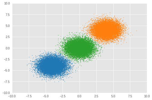
我們可以看到幾乎相同數量的樣本被指派到適當的叢集,且模型也已成功推斷出正確的叢集數量。
4.2. 將不確定性視覺化
在此,我們透過將每個樣本的不確定性視覺化,來檢視分群結果的不確定性。
We calculate uncertainty by using entropy
\[\begin{align*} \text{Uncertainty}_\text{entropy} = -\frac{1}{K}\sum^{K}_{z_i=1}\sum^{O}_{l=1}p(z_i\,|\,x_i,\,\boldsymbol{\theta}_l)\log p(z_i\,|\,x_i,\,\boldsymbol{\theta}_l) \end{align*}\]
在 pSGLD 中,我們將每次迭代的訓練參數值視為其後驗分佈的樣本。因此,我們針對每個參數計算 \(O\) 次迭代值的熵。最終熵值是透過平均所有叢集指派的熵來計算。
# Calculate entropy
posterior_in_exponential = tf.exp(posterior)
uncertainty_in_entropy = tf.reduce_mean(-tf.reduce_sum(
    posterior_in_exponential
    * posterior,
    axis=1), axis=1)

uncertainty_in_entropy_ = sess.run(uncertainty_in_entropy, feed_dict={
    loc_for_posterior: mean_loc_mtx[-sample_size:, :],
    precision_for_posterior: mean_precision_mtx[-sample_size:, :],
    mix_probs_for_posterior: mean_mix_probs_mtx[-sample_size:, :]
})
plt.title('Entropy')
sc = plt.scatter(observations[:, 0],
                 observations[:, 1],
                 1,
                 c=uncertainty_in_entropy_,
                 cmap=plt.cm.viridis_r)
cbar = plt.colorbar(sc,
                    fraction=0.046,
                    pad=0.04,
                    ticks=[uncertainty_in_entropy_.min(),
                           uncertainty_in_entropy_.max()])
cbar.ax.set_yticklabels(['low', 'high'])
cbar.set_label('Uncertainty', rotation=270)
plt.show()
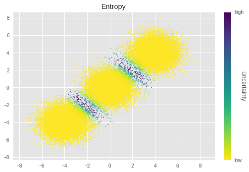
在上圖中,亮度越低表示不確定性越高。我們可以看到叢集邊界附近的樣本具有特別高的不確定性。這在直覺上是正確的,因為這些樣本很難分群。
4.3. 所選混合成分的平均值與尺度
接下來,我們檢視所選叢集的 \(\mu_j\) 和 \(\sigma_j\)。
for idx, numbe_of_samples in zip(idxs, count):
  print(
      'Component id = {}, Number of elements = {}'
      .format(idx, numbe_of_samples))
  print(
      'Mean loc = {}, Mean scale = {}\n'
      .format(mean_loc_[idx, :], mean_precision_[idx, :]))
Component id = 0, Number of elements = 16911
Mean loc = [-4.030 -4.113], Mean scale = [ 0.994  0.972]

Component id = 4, Number of elements = 16645
Mean loc = [ 3.999  4.069], Mean scale = [ 1.038  1.046]

Component id = 5, Number of elements = 16444
Mean loc = [-0.005 -0.023], Mean scale = [ 0.967  1.025]
再次強調,\(\boldsymbol{\mu_j}\) 和 \(\boldsymbol{\sigma_j}\) 接近實際值。
4.4 各混合成分的混合權重
我們也檢視推論出的混合權重。
plt.ylabel('Mean posterior of mixture weight')
plt.xlabel('Component')
plt.bar(range(0, max_cluster_num), mean_mix_probs_)
plt.show()
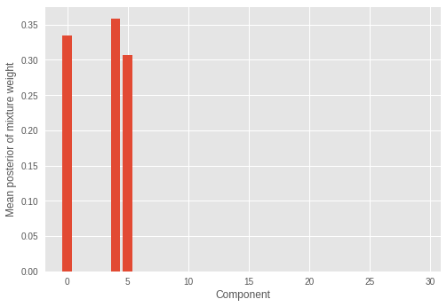
我們看到只有少數(三個)混合成分具有顯著的權重,而其餘權重的數值接近於零。這也表示模型已成功推斷出構成樣本分佈的混合成分的正確數量。
4.5. \(\alpha\) 的收斂性
我們檢視狄利克雷分佈集中參數 \(\alpha\) 的收斂性。
print('Value of inferred alpha = {0:.3f}\n'.format(mean_alpha_[0]))
plt.ylabel('Sample value of alpha')
plt.xlabel('Iteration')
plt.plot(mean_alpha_mtx)
plt.show()
Value of inferred alpha = 0.679
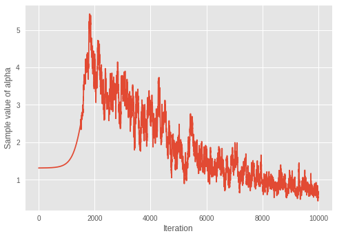
考量到在狄利克雷混合模型中,較小的 \(\alpha\) 會導致較少的預期叢集數量,因此模型似乎正在學習迭代次數中的最佳叢集數量。
4.6. 迭代次數中的推論叢集數量
我們將推論叢集數量在迭代次數中的變化視覺化。
為此,我們推斷迭代次數中的叢集數量。
step = sample_size
num_of_iterations = 50
estimated_num_of_clusters = []
interval = (training_steps - step) // (num_of_iterations - 1)
iterations = np.asarray(range(step, training_steps+1, interval))
for iteration in iterations:
  start_position = iteration-step
  end_position = iteration

  result = sess.run(tf.argmax(
      tf.reduce_mean(posterior, axis=1), axis=1), feed_dict={
          loc_for_posterior:
              mean_loc_mtx[start_position:end_position, :],
          precision_for_posterior:
              mean_precision_mtx[start_position:end_position, :],
          mix_probs_for_posterior:
              mean_mix_probs_mtx[start_position:end_position, :]})

  idxs, count = np.unique(result, return_counts=True)
  estimated_num_of_clusters.append(len(count))
plt.ylabel('Number of inferred clusters')
plt.xlabel('Iteration')
plt.yticks(np.arange(1, max(estimated_num_of_clusters) + 1, 1))
plt.plot(iterations - 1, estimated_num_of_clusters)
plt.show()
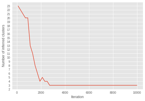
在迭代次數中,叢集數量越來越接近三個。從 \(\alpha\) 在迭代次數中收斂到較小值的結果來看,我們可以看到模型正在成功學習參數,以推斷最佳叢集數量。
有趣的是,我們可以看到推論已在早期迭代中收斂到正確的叢集數量,這與在較晚迭代中收斂的 \(\alpha\) 不同。
4.7. 使用 RMSProp 擬合模型
在本節中,為了瞭解 pSGLD 的蒙地卡羅取樣方案的有效性,我們使用 RMSProp 來擬合模型。我們選擇 RMSProp 進行比較,因為它不包含取樣方案,而 pSGLD 是基於 RMSProp。
# Learning rates and decay
starter_learning_rate_rmsprop = 1e-2
end_learning_rate_rmsprop = 1e-4
decay_steps_rmsprop = 1e4

# Number of training steps
training_steps_rmsprop = 50000

# Mini-batch size
batch_size_rmsprop = 20
# Define trainable variables.
mix_probs_rmsprop = tf.nn.softmax(
    tf.Variable(
        name='mix_probs_rmsprop',
        initial_value=np.ones([max_cluster_num], dtype) / max_cluster_num))

loc_rmsprop = tf.Variable(
    name='loc_rmsprop',
    initial_value=np.zeros([max_cluster_num, dims], dtype)
    + np.random.uniform(
        low=-9, #set around minimum value of sample value
        high=9, #set around maximum value of sample value
        size=[max_cluster_num, dims]))

precision_rmsprop = tf.nn.softplus(tf.Variable(
    name='precision_rmsprop',
    initial_value=
    np.ones([max_cluster_num, dims], dtype=dtype)))

alpha_rmsprop = tf.nn.softplus(tf.Variable(
    name='alpha_rmsprop',
    initial_value=
    np.ones([1], dtype=dtype)))

training_vals_rmsprop =\
    [mix_probs_rmsprop, alpha_rmsprop, loc_rmsprop, precision_rmsprop]

# Prior distributions of the training variables

#Use symmetric Dirichlet prior as finite approximation of Dirichlet process.
rv_symmetric_dirichlet_process_rmsprop = tfd.Dirichlet(
    concentration=np.ones(max_cluster_num, dtype)
    * alpha_rmsprop / max_cluster_num,
    name='rv_sdp_rmsprop')

rv_loc_rmsprop = tfd.Independent(
    tfd.Normal(
        loc=tf.zeros([max_cluster_num, dims], dtype=dtype),
        scale=tf.ones([max_cluster_num, dims], dtype=dtype)),
    reinterpreted_batch_ndims=1,
    name='rv_loc_rmsprop')


rv_precision_rmsprop = tfd.Independent(
    tfd.InverseGamma(
        concentration=np.ones([max_cluster_num, dims], dtype),
        rate=np.ones([max_cluster_num, dims], dtype)),
    reinterpreted_batch_ndims=1,
    name='rv_precision_rmsprop')

rv_alpha_rmsprop = tfd.InverseGamma(
    concentration=np.ones([1], dtype=dtype),
    rate=np.ones([1]),
    name='rv_alpha_rmsprop')

# Define mixture model
rv_observations_rmsprop = tfd.MixtureSameFamily(
    mixture_distribution=tfd.Categorical(probs=mix_probs_rmsprop),
    components_distribution=tfd.MultivariateNormalDiag(
        loc=loc_rmsprop,
        scale_diag=precision_rmsprop))
og_prob_parts_rmsprop = [
    rv_loc_rmsprop.log_prob(loc_rmsprop),
    rv_precision_rmsprop.log_prob(precision_rmsprop),
    rv_alpha_rmsprop.log_prob(alpha_rmsprop),
    rv_symmetric_dirichlet_process_rmsprop
        .log_prob(mix_probs_rmsprop)[..., tf.newaxis],
    rv_observations_rmsprop.log_prob(observations_tensor)
    * num_samples / batch_size
]
joint_log_prob_rmsprop = tf.reduce_sum(
    tf.concat(log_prob_parts_rmsprop, axis=-1), axis=-1)
# Define learning rate scheduling
global_step_rmsprop = tf.Variable(0, trainable=False)
learning_rate = tf.train.polynomial_decay(
    starter_learning_rate_rmsprop,
    global_step_rmsprop, decay_steps_rmsprop,
    end_learning_rate_rmsprop, power=1.)

# Set up the optimizer. Don't forget to set data_size=num_samples.
optimizer_kernel_rmsprop = tf.train.RMSPropOptimizer(
    learning_rate=learning_rate,
    decay=0.99)

train_op_rmsprop = optimizer_kernel_rmsprop.minimize(-joint_log_prob_rmsprop)

init_rmsprop = tf.global_variables_initializer()
sess.run(init_rmsprop)

start = time.time()
for it in range(training_steps_rmsprop):
  [
      _
  ] = sess.run([
      train_op_rmsprop
  ], feed_dict={
      observations_tensor: sess.run(next_batch)})

elapsed_time_rmsprop = time.time() - start
print("RMSProp elapsed_time: {} seconds ({} iterations)"
      .format(elapsed_time_rmsprop, training_steps_rmsprop))
print("pSGLD elapsed_time: {} seconds ({} iterations)"
      .format(elapsed_time_psgld, training_steps))

mix_probs_rmsprop_, alpha_rmsprop_, loc_rmsprop_, precision_rmsprop_ =\
  sess.run(training_vals_rmsprop)
RMSProp elapsed_time: 53.7574200630188 seconds (50000 iterations)
pSGLD elapsed_time: 309.8013095855713 seconds (10000 iterations)
與 pSGLD 相比,雖然 RMSProp 的迭代次數較長,但 RMSProp 的最佳化速度快得多。
接下來,我們檢視分群結果。
cluster_asgmt_rmsprop = sess.run(tf.argmax(
    tf.reduce_mean(posterior, axis=1), axis=1), feed_dict={
        loc_for_posterior: loc_rmsprop_[tf.newaxis, :],
        precision_for_posterior: precision_rmsprop_[tf.newaxis, :],
        mix_probs_for_posterior: mix_probs_rmsprop_[tf.newaxis, :]})

idxs, count = np.unique(cluster_asgmt_rmsprop, return_counts=True)

print('Number of inferred clusters = {}\n'.format(len(count)))
np.set_printoptions(formatter={'float': '{: 0.3f}'.format})

print('Number of elements in each cluster = {}\n'.format(count))

cmap = plt.get_cmap('tab10')
plt.scatter(
    observations[:, 0], observations[:, 1],
    1,
    c=cmap(convert_int_elements_to_consecutive_numbers_in(
        cluster_asgmt_rmsprop)))
plt.axis([-10, 10, -10, 10])
plt.show()
Number of inferred clusters = 4

Number of elements in each cluster = [ 1644 15267 16647 16442]
在我們的實驗中,RMSProp 最佳化並未正確推斷出叢集數量。我們也檢視混合權重。
plt.ylabel('MAP inferece of mixture weight')
plt.xlabel('Component')
plt.bar(range(0, max_cluster_num), mix_probs_rmsprop_)
plt.show()
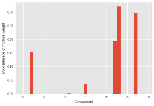
我們可以看到不正確的成分數量具有顯著的混合權重。
儘管最佳化需要更長的時間,但在我們的實驗中,具有蒙地卡羅取樣方案的 pSGLD 表現得更好。
5. 結論
在這份筆記本中,我們已說明如何透過使用 pSGLD 擬合高斯分佈的狄利克雷過程混合模型,對大量樣本進行分群,並同時推斷叢集數量。
實驗已顯示模型成功地對樣本進行分群,並推斷出正確的叢集數量。此外,我們已展示 pSGLD 的蒙地卡羅取樣方案可讓我們將結果中的不確定性視覺化。不僅對樣本進行分群,我們也已看到模型可以推斷出混合成分的正確參數。關於參數與推論叢集數量之間的關係,我們已透過將 \(\alpha\) 收斂性與推論叢集數量之間的關聯性視覺化,來研究模型如何學習參數以控制有效叢集數量。最後,我們已檢視使用 RMSProp 擬合模型的結果。我們已看到 RMSProp 這個不含蒙地卡羅取樣方案的最佳化工具,其運作速度比 pSGLD 快得多,但在分群方面產生的準確性較低。
雖然玩具資料集僅包含 50,000 個樣本,且只有兩個維度,但此處使用的小批量方式最佳化可擴展到更大的資料集。