
|
|
|
 View source on GitHub View source on GitHub
|
|
設定
首先安裝此示範中使用的套件。
pip install -q dm-sonnet
匯入 (tf、tfp 與 adjoint trick 等)
/usr/local/lib/python3.6/dist-packages/statsmodels/tools/_testing.py:19: FutureWarning: pandas.util.testing is deprecated. Use the functions in the public API at pandas.testing instead.
  import pandas.util.testing as tm
用於視覺化的輔助函數
FFJORD 雙射器
在此 colab 中,我們示範 FFJORD 雙射器,最初由 Grathwohl、Will 等人在論文 arxiv link 中提出。
簡而言之,此方法背後的想法是在已知的基礎分佈與資料分佈之間建立對應關係。
為了建立此關聯,我們需要:
- 定義空間 \(\mathcal{Y}\) (基礎分佈定義於此空間) 和資料域空間 \(\mathcal{X}\) 之間的雙射映射 \(\mathcal{T}_{\theta}:\mathbf{x} \rightarrow \mathbf{y}\)、\(\mathcal{T}_{\theta}^{1}:\mathbf{y} \rightarrow \mathbf{x}\)。
- 有效追蹤我們執行的變形,以便將機率概念轉移到 \(\mathcal{X}\)。
第二個條件在以下定義於 \(\mathcal{X}\) 的機率分佈表示式中形式化:
\[ \log p_{\mathbf{x} }(\mathbf{x})=\log p_{\mathbf{y} }(\mathbf{y})-\log \operatorname{det}\left|\frac{\partial \mathcal{T}_{\theta}(\mathbf{y})}{\partial \mathbf{y} }\right| \]
FFJORD 雙射器透過定義轉換來完成此操作:
\[ \mathcal{T_{\theta} }: \mathbf{x} = \mathbf{z}(t_{0}) \rightarrow \mathbf{y} = \mathbf{z}(t_{1}) \quad : \quad \frac{d \mathbf{z} }{dt} = \mathbf{f}(t, \mathbf{z}, \theta) \]
只要描述狀態 \(\mathbf{z}\) 演化的函數 \(\mathbf{f}\) 表現良好,並且可以透過積分以下表達式來計算 log_det_jacobian,則此轉換是可逆的。
\[ \log \operatorname{det}\left|\frac{\partial \mathcal{T}_{\theta}(\mathbf{y})}{\partial \mathbf{y} }\right| = -\int_{t_{0} }^{t_{1} } \operatorname{Tr}\left(\frac{\partial \mathbf{f}(t, \mathbf{z}, \theta)}{\partial \mathbf{z}(t)}\right) d t \]
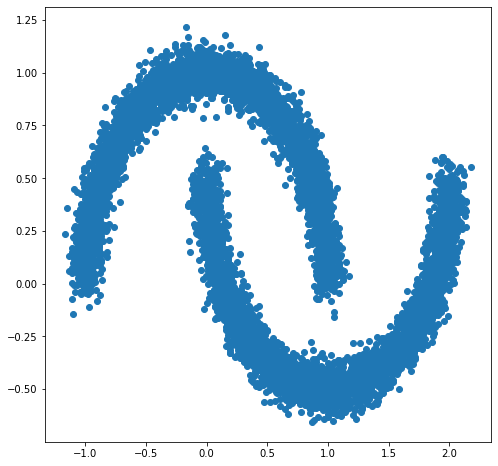
在此示範中,我們將訓練 FFJORD 雙射器,以將高斯分佈扭曲到由 moons 資料集定義的分佈上。這將分 3 個步驟完成:
- 定義基礎分佈
- 定義 FFJORD 雙射器
- 最小化資料集的精確對數似然率
首先,我們載入資料。
資料集
接下來,我們實例化基礎分佈。
base_loc = np.array([0.0, 0.0]).astype(np.float32)
base_sigma = np.array([0.8, 0.8]).astype(np.float32)
base_distribution = tfd.MultivariateNormalDiag(base_loc, base_sigma)
我們使用多層感知器來建模 state_derivative_fn。
雖然對於此資料集而言並非必要,但通常使 state_derivative_fn 依賴於時間是有益的。在這裡,我們透過將 t 串連到網路的輸入來實現這一點。
class MLP_ODE(snt.Module):
  """Multi-layer NN ode_fn."""
  def __init__(self, num_hidden, num_layers, num_output, name='mlp_ode'):
    super(MLP_ODE, self).__init__(name=name)
    self._num_hidden = num_hidden
    self._num_output = num_output
    self._num_layers = num_layers
    self._modules = []
    for _ in range(self._num_layers - 1):
      self._modules.append(snt.Linear(self._num_hidden))
      self._modules.append(tf.math.tanh)
    self._modules.append(snt.Linear(self._num_output))
    self._model = snt.Sequential(self._modules)

  def __call__(self, t, inputs):
    inputs = tf.concat([tf.broadcast_to(t, inputs.shape), inputs], -1)
    return self._model(inputs)
模型與訓練參數
現在我們建構 FFJORD 雙射器的堆疊。每個雙射器都提供 ode_solve_fn 和 trace_augmentation_fn 以及其自己的 state_derivative_fn 模型,以便它們代表一系列不同的轉換。
建構雙射器
現在我們可以使用 TransformedDistribution,這是使用 stacked_ffjord 雙射器扭曲 base_distribution 的結果。
transformed_distribution = tfd.TransformedDistribution(
    distribution=base_distribution, bijector=stacked_ffjord)
現在我們定義訓練程序。我們只需最小化資料的負對數似然率。
訓練
樣本
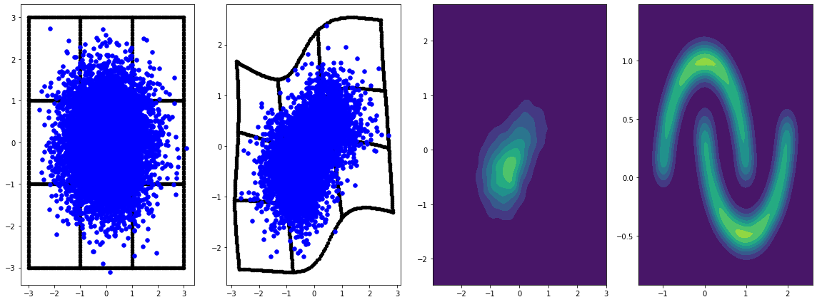
繪製來自基礎分佈和轉換分佈的樣本。
evaluation_samples = []
base_samples, transformed_samples = get_samples()
transformed_grid = get_transformed_grid()
evaluation_samples.append((base_samples, transformed_samples, transformed_grid))
WARNING:tensorflow:From /usr/local/lib/python3.6/dist-packages/tensorflow/python/ops/resource_variable_ops.py:1817: calling BaseResourceVariable.__init__ (from tensorflow.python.ops.resource_variable_ops) with constraint is deprecated and will be removed in a future version.
Instructions for updating:
If using Keras pass *_constraint arguments to layers.
panel_id = 0
panel_data = evaluation_samples[panel_id]
fig, axarray = plt.subplots(
  1, 4, figsize=(16, 6))
plot_panel(
    grid, panel_data[0], panel_data[2], panel_data[1], moons, axarray, False)
plt.tight_layout()
learning_rate = tf.Variable(LR, trainable=False)
optimizer = snt.optimizers.Adam(learning_rate)

for epoch in tqdm.trange(NUM_EPOCHS // 2):
  base_samples, transformed_samples = get_samples()
  transformed_grid = get_transformed_grid()
  evaluation_samples.append(
      (base_samples, transformed_samples, transformed_grid))
  for batch in moons_ds:
    _ = train_step(optimizer, batch)
0%|          | 0/40 [00:00<?, ?it/s]
WARNING:tensorflow:From /usr/local/lib/python3.6/dist-packages/tensorflow_probability/python/math/ode/base.py:350: calling while_loop_v2 (from tensorflow.python.ops.control_flow_ops) with back_prop=False is deprecated and will be removed in a future version.
Instructions for updating:
back_prop=False is deprecated. Consider using tf.stop_gradient instead.
Instead of:
results = tf.while_loop(c, b, vars, back_prop=False)
Use:
results = tf.nest.map_structure(tf.stop_gradient, tf.while_loop(c, b, vars))
100%|██████████| 40/40 [07:00<00:00, 10.52s/it]
panel_id = -1
panel_data = evaluation_samples[panel_id]
fig, axarray = plt.subplots(
  1, 4, figsize=(16, 6))
plot_panel(grid, panel_data[0], panel_data[2], panel_data[1], moons, axarray)
plt.tight_layout()
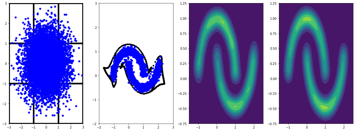
使用學習率進行更長時間的訓練可帶來進一步的改進。
此範例未涵蓋,FFJORD 雙射器支援 Hutchinson 的隨機跡線估計。特定的估計器可以透過 trace_augmentation_fn 提供。同樣地,可以透過定義自訂 ode_solve_fn 來使用替代積分器。