
|
|
|
 在 GitHub 上檢視原始碼 在 GitHub 上檢視原始碼
|
|
八所學校問題 (Rubin 1981) 考量在八所學校平行進行的 SAT 指導計畫的成效。這已成為一個經典問題 (Bayesian Data Analysis、Stan),說明階層式模型對於在可交換群組之間分享資訊的實用性。
以下實作是 Edward 1.0 教學課程的改編版本。
匯入
import matplotlib.pyplot as plt
import numpy as np
import seaborn as sns

import tensorflow.compat.v2 as tf
import tensorflow_probability as tfp
from tensorflow_probability import distributions as tfd
import warnings

tf.enable_v2_behavior()

plt.style.use("ggplot")
warnings.filterwarnings('ignore')
資料
出自 Bayesian Data Analysis 第 5.5 節 (Gelman et al. 2013)
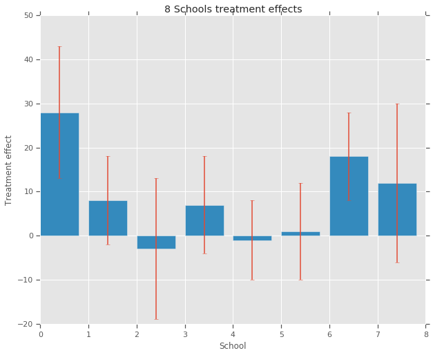
教育測驗服務中心進行了一項研究,旨在分析八所高中各自的 SAT-V (學術性向測驗 - 語文) 特殊指導計畫的成效。結果變數是每項研究中 SAT-V 的特殊管理分數,這是一項由教育測驗服務中心管理、用於協助大學做出入學決定的標準化多項選擇題測驗;分數介於 200 到 800 之間,平均約為 500,標準差約為 100。SAT 測驗旨在抵抗專門針對提升測驗表現的短期努力;相反地,它們旨在反映多年教育所習得的知識和培養的能力。然而,本研究中的八所學校都認為其短期指導計畫在提高 SAT 分數方面非常成功。此外,沒有先前的理由可以相信這八個計畫中的任何一個比其他計畫更有效,或者某些計畫的效果彼此之間比其他計畫更相似。
針對八所學校中的每一所學校 (J = 8),我們都有一個估計的處理效應 \(y_j\) 和效應估計的標準誤 \(\sigma_j\)。研究中的處理效應是透過對處理組進行線性迴歸,並使用 PSAT-M 和 PSAT-V 分數作為控制變數而獲得的。由於沒有先前的信念認為任何學校更相似或更不相似,或者任何指導計畫會更有效,因此我們可以將處理效應視為 可交換。
num_schools = 8  # number of schools
treatment_effects = np.array(
    [28, 8, -3, 7, -1, 1, 18, 12], dtype=np.float32)  # treatment effects
treatment_stddevs = np.array(
    [15, 10, 16, 11, 9, 11, 10, 18], dtype=np.float32)  # treatment SE

fig, ax = plt.subplots()
plt.bar(range(num_schools), treatment_effects, yerr=treatment_stddevs)
plt.title("8 Schools treatment effects")
plt.xlabel("School")
plt.ylabel("Treatment effect")
fig.set_size_inches(10, 8)
plt.show()
模型
為了擷取資料,我們使用階層式常態模型。它遵循生成過程:
\[ \begin{align*} \mu &\sim \text{Normal}(\text{loc}{=}0,\ \text{scale}{=}10) \\ \log\tau &\sim \text{Normal}(\text{loc}{=}5,\ \text{scale}{=}1) \\ \text{for } & i=1\ldots 8:\\ & \theta_i \sim \text{Normal}\left(\text{loc}{=}\mu,\ \text{scale}{=}\tau \right) \\ & y_i \sim \text{Normal}\left(\text{loc}{=}\theta_i,\ \text{scale}{=}\sigma_i \right) \end{align*} \]
其中 \(\mu\) 代表先驗平均處理效應,\(\tau\) 控制學校之間的變異數大小。\(y_i\) 和 \(\sigma_i\) 是觀察值。當 \(\tau \rightarrow \infty\) 時,模型會趨近於無共用模型,也就是說,每個學校的處理效應估計值可以更獨立。當 \(\tau \rightarrow 0\) 時,模型會趨近於完全共用模型,也就是說,所有學校的處理效應都更接近群組平均值 \(\mu\)。為了限制標準差為正數,我們從對數常態分配中抽取 \(\tau\) (這相當於從常態分配中抽取 \(log(\tau)\))。
根據「使用分歧診斷偏差推論」,我們將上述模型轉換為等效的非中心模型
\[ \begin{align*} \mu &\sim \text{Normal}(\text{loc}{=}0,\ \text{scale}{=}10) \\ \log\tau &\sim \text{Normal}(\text{loc}{=}5,\ \text{scale}{=}1) \\ \text{for } & i=1\ldots 8:\\ & \theta_i' \sim \text{Normal}\left(\text{loc}{=}0,\ \text{scale}{=}1 \right) \\ & \theta_i = \mu + \tau \theta_i' \\ & y_i \sim \text{Normal}\left(\text{loc}{=}\theta_i,\ \text{scale}{=}\sigma_i \right) \end{align*} \]
我們將此模型具體化為 JointDistributionSequential 執行個體
model = tfd.JointDistributionSequential([
  tfd.Normal(loc=0., scale=10., name="avg_effect"),  # `mu` above
  tfd.Normal(loc=5., scale=1., name="avg_stddev"),  # `log(tau)` above
  tfd.Independent(tfd.Normal(loc=tf.zeros(num_schools),
                             scale=tf.ones(num_schools),
                             name="school_effects_standard"),  # `theta_prime`
                  reinterpreted_batch_ndims=1),
  lambda school_effects_standard, avg_stddev, avg_effect: (
      tfd.Independent(tfd.Normal(loc=(avg_effect[..., tf.newaxis] +
                                      tf.exp(avg_stddev[..., tf.newaxis]) *
                                      school_effects_standard),  # `theta` above
                                 scale=treatment_stddevs),
                      name="treatment_effects",  # `y` above
                      reinterpreted_batch_ndims=1))
])

def target_log_prob_fn(avg_effect, avg_stddev, school_effects_standard):
  """Unnormalized target density as a function of states."""
  return model.log_prob((
      avg_effect, avg_stddev, school_effects_standard, treatment_effects))
貝氏推論
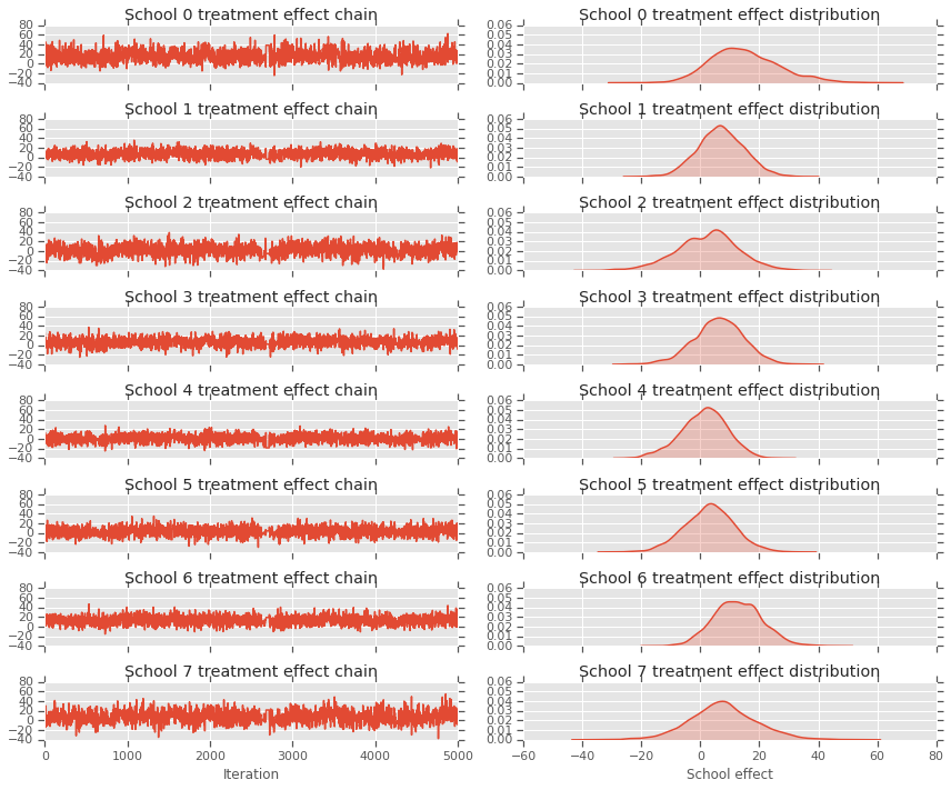
在給定資料的情況下,我們執行哈密頓蒙地卡羅 (HMC) 來計算模型參數的後驗分配。
num_results = 5000
num_burnin_steps = 3000

# Improve performance by tracing the sampler using `tf.function`
# and compiling it using XLA.
@tf.function(autograph=False, jit_compile=True)
def do_sampling():
  return tfp.mcmc.sample_chain(
      num_results=num_results,
      num_burnin_steps=num_burnin_steps,
      current_state=[
          tf.zeros([], name='init_avg_effect'),
          tf.zeros([], name='init_avg_stddev'),
          tf.ones([num_schools], name='init_school_effects_standard'),
      ],
      kernel=tfp.mcmc.HamiltonianMonteCarlo(
          target_log_prob_fn=target_log_prob_fn,
          step_size=0.4,
          num_leapfrog_steps=3))

states, kernel_results = do_sampling()

avg_effect, avg_stddev, school_effects_standard = states

school_effects_samples = (
    avg_effect[:, np.newaxis] +
    np.exp(avg_stddev)[:, np.newaxis] * school_effects_standard)

num_accepted = np.sum(kernel_results.is_accepted)
print('Acceptance rate: {}'.format(num_accepted / num_results))
Acceptance rate: 0.5974
fig, axes = plt.subplots(8, 2, sharex='col', sharey='col')
fig.set_size_inches(12, 10)
for i in range(num_schools):
  axes[i][0].plot(school_effects_samples[:,i].numpy())
  axes[i][0].title.set_text("School {} treatment effect chain".format(i))
  sns.kdeplot(school_effects_samples[:,i].numpy(), ax=axes[i][1], shade=True)
  axes[i][1].title.set_text("School {} treatment effect distribution".format(i))
axes[num_schools - 1][0].set_xlabel("Iteration")
axes[num_schools - 1][1].set_xlabel("School effect")
fig.tight_layout()
plt.show()
print("E[avg_effect] = {}".format(np.mean(avg_effect)))
print("E[avg_stddev] = {}".format(np.mean(avg_stddev)))
print("E[school_effects_standard] =")
print(np.mean(school_effects_standard[:, ]))
print("E[school_effects] =")
print(np.mean(school_effects_samples[:, ], axis=0))
E[avg_effect] = 5.57183933258
E[avg_stddev] = 2.47738981247
E[school_effects_standard] =
0.08509017
E[school_effects] =
[15.0051     7.103311   2.4552586  6.2744603  1.3364682  3.1125953
 12.762501   7.743602 ]
# Compute the 95% interval for school_effects
school_effects_low = np.array([
    np.percentile(school_effects_samples[:, i], 2.5) for i in range(num_schools)
])
school_effects_med = np.array([
    np.percentile(school_effects_samples[:, i], 50) for i in range(num_schools)
])
school_effects_hi = np.array([
    np.percentile(school_effects_samples[:, i], 97.5)
    for i in range(num_schools)
])
fig, ax = plt.subplots(nrows=1, ncols=1, sharex=True)
ax.scatter(np.array(range(num_schools)), school_effects_med, color='red', s=60)
ax.scatter(
    np.array(range(num_schools)) + 0.1, treatment_effects, color='blue', s=60)

plt.plot([-0.2, 7.4], [np.mean(avg_effect),
                       np.mean(avg_effect)], 'k', linestyle='--')

ax.errorbar(
    np.array(range(8)),
    school_effects_med,
    yerr=[
        school_effects_med - school_effects_low,
        school_effects_hi - school_effects_med
    ],
    fmt='none')

ax.legend(('avg_effect', 'HMC', 'Observed effect'), fontsize=14)

plt.xlabel('School')
plt.ylabel('Treatment effect')
plt.title('HMC estimated school treatment effects vs. observed data')
fig.set_size_inches(10, 8)
plt.show()
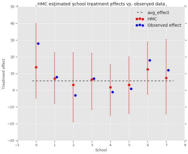
我們可以觀察到上述朝向群組 avg_effect 的收縮。
print("Inferred posterior mean: {0:.2f}".format(
    np.mean(school_effects_samples[:,])))
print("Inferred posterior mean se: {0:.2f}".format(
    np.std(school_effects_samples[:,])))
Inferred posterior mean: 6.97
Inferred posterior mean se: 10.41
評論
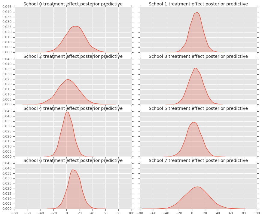
為了取得後驗預測分配,即在給定觀測資料 \(y\) 的情況下,新資料 \(y^*\) 的模型
\[ p(y^*|y) \propto \int_\theta p(y^* | \theta)p(\theta |y)d\theta\]
我們會覆寫模型中隨機變數的值,將其設為後驗分配的平均值,並從該模型取樣以產生新資料 \(y^*\)。
sample_shape = [5000]

_, _, _, predictive_treatment_effects = model.sample(
    value=(tf.broadcast_to(np.mean(avg_effect, 0), sample_shape),
           tf.broadcast_to(np.mean(avg_stddev, 0), sample_shape),
           tf.broadcast_to(np.mean(school_effects_standard, 0),
                           sample_shape + [num_schools]),
           None))
fig, axes = plt.subplots(4, 2, sharex=True, sharey=True)
fig.set_size_inches(12, 10)
fig.tight_layout()
for i, ax in enumerate(axes):
  sns.kdeplot(predictive_treatment_effects[:, 2*i].numpy(),
              ax=ax[0], shade=True)
  ax[0].title.set_text(
      "School {} treatment effect posterior predictive".format(2*i))
  sns.kdeplot(predictive_treatment_effects[:, 2*i + 1].numpy(),
              ax=ax[1], shade=True)
  ax[1].title.set_text(
      "School {} treatment effect posterior predictive".format(2*i + 1))
plt.show()
# The mean predicted treatment effects for each of the eight schools.
prediction = np.mean(predictive_treatment_effects, axis=0)
我們可以查看處理效應資料與模型後驗預測之間的殘差。這些殘差與上面的圖表對應,圖表顯示估計效應朝向母體平均值的收縮。
treatment_effects - prediction
array([14.905351 ,  1.2838383, -5.6966295,  0.8327627, -2.3356671,
       -2.0363257,  5.997898 ,  4.3731265], dtype=float32)
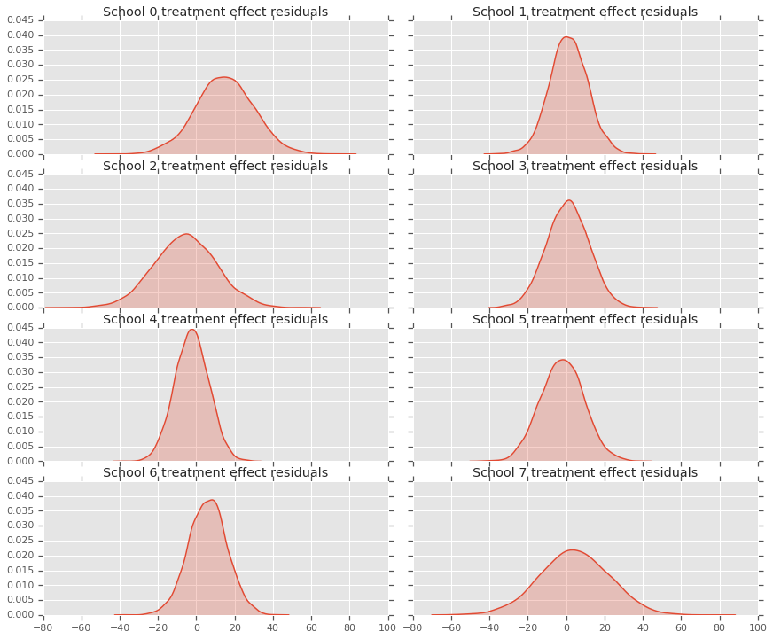
由於我們有每所學校的預測分配,因此我們也可以考量殘差的分配。
residuals = treatment_effects - predictive_treatment_effects
fig, axes = plt.subplots(4, 2, sharex=True, sharey=True)
fig.set_size_inches(12, 10)
fig.tight_layout()
for i, ax in enumerate(axes):
  sns.kdeplot(residuals[:, 2*i].numpy(), ax=ax[0], shade=True)
  ax[0].title.set_text(
      "School {} treatment effect residuals".format(2*i))
  sns.kdeplot(residuals[:, 2*i + 1].numpy(), ax=ax[1], shade=True)
  ax[1].title.set_text(
      "School {} treatment effect residuals".format(2*i + 1))
plt.show()
致謝
本教學課程最初以 Edward 1.0 (來源) 編寫。我們感謝所有為撰寫和修訂該版本做出貢獻的人員。
參考資料
- Donald B. Rubin. Estimation in parallel randomized experiments. Journal of Educational Statistics, 6(4):377-401, 1981.
- Andrew Gelman, John Carlin, Hal Stern, David Dunson, Aki Vehtari, and Donald Rubin. Bayesian Data Analysis, Third Edition. Chapman and Hall/CRC, 2013.