
|
|
|
 在 GitHub 上檢視原始碼 在 GitHub 上檢視原始碼
|
|
JAX 上的 TensorFlow Probability (TFP) 現在具備分散式數值運算工具。為了擴展到大量加速器,這些工具的建構基礎是使用「單一程式多資料」範例 (簡稱 SPMD) 撰寫程式碼。
在本筆記本中,我們將說明如何「以 SPMD 思考」,並介紹新的 TFP 抽象概念,以便擴展到 TPU Pod 或 GPU 叢集等組態。如果您自行執行此程式碼,請務必選取 TPU 執行階段。
我們先安裝最新版本的 TFP、JAX 和 TF。
安裝
我們將匯入一些通用程式庫,以及一些 JAX 公用程式。
設定與匯入
INFO:tensorflow:Enabling eager execution
INFO:tensorflow:Enabling v2 tensorshape
INFO:tensorflow:Enabling resource variables
INFO:tensorflow:Enabling tensor equality
INFO:tensorflow:Enabling control flow v2
我們也會設定一些方便的 TFP 別名。新的抽象概念目前在 tfp.experimental.distribute 和 tfp.experimental.mcmc 中提供。
tfd = tfp.distributions
tfb = tfp.bijectors
tfm = tfp.mcmc
tfed = tfp.experimental.distribute
tfde = tfp.experimental.distributions
tfem = tfp.experimental.mcmc

Root = tfed.JointDistributionCoroutine.Root
若要將筆記本連線至 TPU,我們使用 JAX 的以下協助程式。為了確認已連線,我們印出裝置數量,應為八個。
from jax.tools import colab_tpu
colab_tpu.setup_tpu()
print(f'Found {jax.device_count()} devices')
Found 8 devices
jax.pmap 快速入門
連線至 TPU 後,我們可以存取八個裝置。不過,當我們積極執行 JAX 程式碼時,JAX 預設只在一個裝置上執行運算。
跨多個裝置執行運算最簡單的方式是對函式進行對應,讓每個裝置執行對應的一個索引。JAX 提供 jax.pmap (「平行對應」) 轉換,可將函式轉換為跨多個裝置對應函式的函式。
在以下範例中,我們建立大小為 8 的陣列 (以符合可用裝置數量),並對將 5 加到陣列的函式進行對應。
xs = jnp.arange(8.)
out = jax.pmap(lambda x: x + 5.)(xs)
print(type(out), out)
<class 'jax.interpreters.pxla.ShardedDeviceArray'> [ 5. 6. 7. 8. 9. 10. 11. 12.]
請注意,我們會收到 ShardedDeviceArray 類型,表示輸出陣列在實體上跨裝置分割。
jax.pmap 在語意上類似於對應,但有一些重要選項可修改其行為。根據預設,pmap 假設函式的所有輸入都經過對應,但我們可以透過 in_axes 引數修改此行為。
xs = jnp.arange(8.)
y = 5.
# Map over the 0-axis of `xs` and don't map over `y`
out = jax.pmap(lambda x, y: x + y, in_axes=(0, None))(xs, y)
print(out)
[ 5. 6. 7. 8. 9. 10. 11. 12.]
類似地,pmap 的 out_axes 引數決定是否傳回每個裝置上的值。將 out_axes 設定為 None 會自動傳回第 1 個裝置上的值,而且只有在我們確信每個裝置上的值都相同時才應使用。
xs = jnp.ones(8) # Value is the same on each device
out = jax.pmap(lambda x: x + 1, out_axes=None)(xs)
print(out)
2.0
當我們想要執行的動作不容易以對應的純函式表示時,會發生什麼事?例如,如果我們想要對我們對應的軸執行總和,該怎麼辦?JAX 提供「collectives」(跨裝置通訊的函式),以便撰寫更有趣且更複雜的分散式程式。為了瞭解其運作方式,我們將介紹 SPMD。
什麼是 SPMD?
單一程式多資料 (SPMD) 是一種並行程式設計模型,其中單一程式 (即相同的程式碼) 會在多個裝置上同時執行,但每個執行中程式的輸入可能不同。
如果我們的程式是其輸入的簡單函式 (即類似 x + 5),則在 SPMD 中執行程式只是將其對應到不同的資料,就像我們稍早使用 jax.pmap 所做的一樣。不過,我們不僅可以「對應」函式。JAX 提供「collectives」,這些函式可在多個裝置之間通訊。
例如,我們可能想要計算所有裝置上某個數量的總和。在執行此操作之前,我們需要為 pmap 中對應的軸指派名稱。然後,我們使用 lax.psum (「平行總和」) 函式在多個裝置之間執行總和,確保我們識別要加總的已命名軸。
def f(x):
  out = lax.psum(x, axis_name='i')
  return out
xs = jnp.arange(8.) # Length of array matches number of devices
jax.pmap(f, axis_name='i')(xs)
ShardedDeviceArray([28., 28., 28., 28., 28., 28., 28., 28.], dtype=float32)
psum collective 會彙總每個裝置上 x 的值,並在對應中同步其值,即每個裝置上的 out 都是 28。我們不再執行簡單的「對應」,而是執行 SPMD 程式,其中每個裝置的運算現在都可以與其他裝置上的相同運算互動,儘管是以有限的方式使用 collectives。在此情境中,我們可以使用 out_axes = None,因為 psum 會同步值。
def f(x):
  out = lax.psum(x, axis_name='i')
  return out
jax.pmap(f, axis_name='i', out_axes=None)(jnp.arange(8.))
ShardedDeviceArray(28., dtype=float32)
SPMD 讓我們能夠撰寫一個程式,在任何 TPU 組態中的每個裝置上同時執行。用於在 8 個 TPU 核心上執行機器學習的相同程式碼,可用於可能具有數百到數千個核心的 TPU Pod!如需關於 jax.pmap 和 SPMD 的更詳細教學課程,您可以參閱 JAX 101 教學課程。
大規模 MCMC
在本筆記本中,我們著重於使用馬可夫鏈蒙地卡羅 (MCMC) 方法進行貝氏推論。我們可以使用多種方式利用多個裝置進行 MCMC,但在本筆記本中,我們將著重於兩種方式
- 在不同裝置上執行獨立的馬可夫鏈。這種情況相當簡單,而且可以使用原始 TFP 完成。
- 跨裝置分割資料集。這種情況稍微複雜一些,而且需要最近新增的 TFP 機制。
獨立鏈
假設我們想要使用 MCMC 對問題執行貝氏推論,並想要跨多個裝置平行執行多個鏈 (例如每個裝置上 2 個)。這結果是一個我們可以跨裝置「對應」的程式,即不需要 collectives 的程式。為了確保每個程式執行不同的馬可夫鏈 (而不是執行相同的鏈),我們將不同的隨機種子值傳遞給每個裝置。
讓我們在從 2D 高斯分配取樣的玩具問題上試試看。我們可以立即使用 TFP 現有的 MCMC 功能。一般而言,我們嘗試將大部分邏輯放在對應的函式內,以更明確地區分在所有裝置上執行的內容與僅在第一個裝置上執行的內容。
def run(seed):
  target_log_prob = tfd.Sample(tfd.Normal(0., 1.), 2).log_prob

  initial_state = jnp.zeros([2, 2]) # 2 chains
  kernel = tfm.HamiltonianMonteCarlo(target_log_prob, 1e-1, 10)
  def trace_fn(state, pkr):
    return target_log_prob(state)

  states, log_prob = tfm.sample_chain(
    num_results=1000,
    num_burnin_steps=1000,
    kernel=kernel,
    current_state=initial_state,
    trace_fn=trace_fn,
    seed=seed
  )
  return states, log_prob
就其本身而言,run 函式會接收無狀態隨機種子 (若要瞭解無狀態隨機性如何運作,您可以閱讀 JAX 上的 TFP 筆記本或參閱 JAX 101 教學課程)。跨不同種子對 run 進行對應,將會導致執行多個獨立的馬可夫鏈。
states, log_probs = jax.pmap(run)(random.split(random.PRNGKey(0), 8))
print(states.shape, log_probs.shape)
# states is (8 devices, 1000 samples, 2 chains, 2 dimensions)
# log_prob is (8 devices, 1000 samples, 2 chains)
(8, 1000, 2, 2) (8, 1000, 2)
請注意,我們現在有一個額外的軸對應於每個裝置。我們可以重新排列維度並將其扁平化,以取得 16 個鏈的軸。
states = states.transpose([0, 2, 1, 3]).reshape([-1, 1000, 2])
log_probs = log_probs.transpose([0, 2, 1]).reshape([-1, 1000])
fig, ax = plt.subplots(1, 2, figsize=(10, 5))
ax[0].plot(log_probs.T, alpha=0.4)
ax[1].scatter(*states.reshape([-1, 2]).T, alpha=0.1)
plt.show()
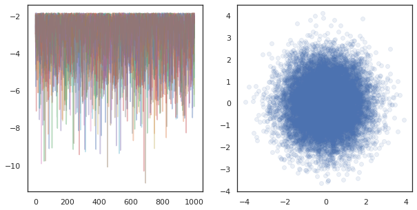
在多個裝置上執行獨立鏈時,就像對使用 tfp.mcmc 的函式進行 pmap 一樣簡單,確保我們將不同的隨機種子值傳遞給每個裝置。
分割資料
當我們執行 MCMC 時,目標分配通常是透過以資料集為條件取得的後驗分配,而計算未正規化的對數密度涉及加總每個觀察資料的概似。
對於非常大的資料集,即使在單一裝置上執行一個鏈也可能非常昂貴。不過,當我們可以存取多個裝置時,我們可以跨裝置分割資料集,以更充分利用我們可用的運算資源。
如果我們想要使用分割資料集執行 MCMC,我們需要確保在每個裝置上計算的未正規化對數密度代表總計,即所有資料的密度,否則每個裝置都會使用自己不正確的目標分配執行 MCMC。為此,TFP 現在具備新工具 (即 tfp.experimental.distribute 和 tfp.experimental.mcmc),可讓您計算「分割」對數機率並使用 MCMC 執行這些機率。
分割分配
TFP 現在提供的用於計算分割對數機率的核心抽象概念是 Sharded 中繼分配,它會將分配作為輸入,並傳回在 SPMD 環境中執行時具有特定屬性的新分配。Sharded 位於 tfp.experimental.distribute 中。
直覺上,Sharded 分配對應於一組已「分割」到多個裝置的隨機變數。在每個裝置上,它們會產生不同的樣本,而且可以個別具有不同的對數密度。或者,Sharded 分配對應於圖形模型術語中的「板」,其中板大小是裝置數量。
取樣 Sharded 分配
如果我們在使用相同種子的每個裝置上 pmap 的程式中從 Normal 分配取樣,我們會在每個裝置上取得相同的樣本。我們可以將以下函式視為取樣跨裝置同步的單一隨機變數。
# `pmap` expects at least one value to be mapped over, so we provide a dummy one
def f(seed, _):
  return tfd.Normal(0., 1.).sample(seed=seed)
jax.pmap(f, in_axes=(None, 0))(random.PRNGKey(0), jnp.arange(8.))
ShardedDeviceArray([-0.20584236, -0.20584236, -0.20584236, -0.20584236,
                    -0.20584236, -0.20584236, -0.20584236, -0.20584236],                   dtype=float32)
如果我們使用 tfed.Sharded 包裝 tfd.Normal(0., 1.),則在邏輯上我們現在有八個不同的隨機變數 (每個裝置上一個),因此即使傳入相同的種子,也會為每個變數產生不同的樣本。
def f(seed, _):
  return tfed.Sharded(tfd.Normal(0., 1.), shard_axis_name='i').sample(seed=seed)
jax.pmap(f, in_axes=(None, 0), axis_name='i')(random.PRNGKey(0), jnp.arange(8.))
ShardedDeviceArray([ 1.2152631 ,  0.7818249 ,  0.32549605,  0.6828047 ,
                     1.3973192 , -0.57830244,  0.37862757,  2.7706041 ],                   dtype=float32)
在單一裝置上,此分配的對等表示法只是 8 個獨立的常態樣本。即使樣本的值會不同 (tfed.Sharded 以稍微不同的方式執行虛擬隨機數產生),但它們都代表相同的分配。
dist = tfd.Sample(tfd.Normal(0., 1.), jax.device_count())
dist.sample(seed=random.PRNGKey(0))
DeviceArray([ 0.08086783, -0.38624594, -0.3756545 ,  1.668957  ,
             -1.2758069 ,  2.1192007 , -0.85821325,  1.1305912 ],            dtype=float32)
取得 Sharded 分配的對數密度
讓我們看看在 SPMD 環境中計算常規分配樣本的對數密度時會發生什麼事。
def f(seed, _):
  dist = tfd.Normal(0., 1.)
  x = dist.sample(seed=seed)
  return x, dist.log_prob(x)
jax.pmap(f, in_axes=(None, 0))(random.PRNGKey(0), jnp.arange(8.))
(ShardedDeviceArray([-0.20584236, -0.20584236, -0.20584236, -0.20584236,
                     -0.20584236, -0.20584236, -0.20584236, -0.20584236],                   dtype=float32),
 ShardedDeviceArray([-0.94012403, -0.94012403, -0.94012403, -0.94012403,
                     -0.94012403, -0.94012403, -0.94012403, -0.94012403],                   dtype=float32))
每個裝置上的樣本都相同,因此我們也在每個裝置上計算相同的密度。直覺上,這裡我們只有單一常態分配變數的分配。
使用 Sharded 分配,我們有 8 個隨機變數的分配,因此當我們計算樣本的 log_prob 時,我們會跨裝置加總每個個別的對數密度。(您可能會注意到,此總計 log_prob 值大於上方計算的 singleton log_prob。)
def f(seed, _):
  dist = tfed.Sharded(tfd.Normal(0., 1.), shard_axis_name='i')
  x = dist.sample(seed=seed)
  return x, dist.log_prob(x)
sample, log_prob = jax.pmap(f, in_axes=(None, 0), axis_name='i')(
    random.PRNGKey(0), jnp.arange(8.))
print('Sample:', sample)
print('Log Prob:', log_prob)
Sample: [ 1.2152631   0.7818249   0.32549605  0.6828047   1.3973192  -0.57830244
  0.37862757  2.7706041 ]
Log Prob: [-13.7349205 -13.7349205 -13.7349205 -13.7349205 -13.7349205 -13.7349205
 -13.7349205 -13.7349205]
對等的「未分割」分配會產生相同的對數密度。
dist = tfd.Sample(tfd.Normal(0., 1.), jax.device_count())
dist.log_prob(sample)
DeviceArray(-13.7349205, dtype=float32)
Sharded 分配會從每個裝置上的 sample 產生不同的值,但在每個裝置上取得相同的 log_prob 值。這裡發生了什麼事?Sharded 分配會在內部執行 psum,以確保 log_prob 值在多個裝置之間同步。我們為什麼需要這種行為?如果我們在每個裝置上執行相同的 MCMC 鏈,我們會希望每個裝置上的 target_log_prob 都相同,即使運算中的某些隨機變數跨裝置分割也一樣。
此外,Sharded 分配可確保跨裝置的梯度正確,以確保 HMC 等演算法 (將對數密度函式的梯度作為轉換函式的一部分) 產生適當的樣本。
分割 JointDistribution
我們可以使用 JointDistribution (JD) 建立具有多個 Sharded 隨機變數的模型。不幸的是,Sharded 分配無法安全地與原始 tfd.JointDistribution 一起使用,但 tfp.experimental.distribute 匯出「修補」的 JD,其行為會類似於 Sharded 分配。
def f(seed, _):
  dist = tfed.JointDistributionSequential([
    tfd.Normal(0., 1.),
    tfed.Sharded(tfd.Normal(0., 1.), shard_axis_name='i'),
  ])
  x = dist.sample(seed=seed)
  return x, dist.log_prob(x)
jax.pmap(f, in_axes=(None, 0), axis_name='i')(random.PRNGKey(0), jnp.arange(8.))
([ShardedDeviceArray([1.6121525, 1.6121525, 1.6121525, 1.6121525, 1.6121525,
                      1.6121525, 1.6121525, 1.6121525], dtype=float32),
  ShardedDeviceArray([ 0.8690128 , -0.83167845,  1.2209264 ,  0.88412696,
                       0.76478404, -0.66208494, -0.0129658 ,  0.7391483 ],                   dtype=float32)],
 ShardedDeviceArray([-12.214451, -12.214451, -12.214451, -12.214451,
                     -12.214451, -12.214451, -12.214451, -12.214451],                   dtype=float32))
這些分割 JD 可以同時具有 Sharded 和原始 TFP 分配作為組件。對於未分割的分配,我們在每個裝置上取得相同的樣本,而對於分割的分配,我們取得不同的樣本。每個裝置上的 log_prob 也會同步。
使用 Sharded 分配的 MCMC
我們應如何在 MCMC 的環境中思考 Sharded 分配?如果我們有可以表示為 JointDistribution 的生成模型,我們可以選取該模型的某些軸來「分割」。通常,模型中的一個隨機變數會對應於觀察到的資料,而且如果我們有想要跨裝置分割的大型資料集,我們會希望與資料點相關聯的變數也分割。我們也可能具有與我們分割的觀察結果一對一的「本機」隨機變數,因此我們也必須分割這些隨機變數。
在本節中,我們將說明搭配 TFP MCMC 使用 Sharded 分配的範例。我們將從較簡單的貝氏邏輯迴歸範例開始,並以矩陣分解範例結束,目標是示範 distribute 程式庫的一些使用案例。
範例:MNIST 的貝氏邏輯迴歸
我們想要對大型資料集執行貝氏邏輯迴歸;模型在迴歸權重上具有先驗 \(p(\theta)\),以及針對所有資料 \(\{x_i, y_i\}_{i = 1}^N\) 加總的概似 \(p(y_i | \theta, x_i)\),以取得總聯合對數密度。如果我們分割資料,我們會分割模型中觀察到的隨機變數 \(x_i\) 和 \(y_i\)。
我們將以下貝氏邏輯迴歸模型用於 MNIST 分類
\[ \begin{align*} w &\sim \mathcal{N}(0, 1) \\ b &\sim \mathcal{N}(0, 1) \\ y_i | w, b, x_i &\sim \textrm{Categorical}(w^T x_i + b) \end{align*} \]
讓我們使用 TensorFlow Datasets 載入 MNIST。
mnist = tfds.as_numpy(tfds.load('mnist', batch_size=-1))
raw_train_images, train_labels = mnist['train']['image'], mnist['train']['label']
train_images = raw_train_images.reshape([raw_train_images.shape[0], -1]) / 255.

raw_test_images, test_labels = mnist['test']['image'], mnist['test']['label']
test_images = raw_test_images.reshape([raw_test_images.shape[0], -1]) / 255.
Downloading and preparing dataset mnist/3.0.1 (download: 11.06 MiB, generated: 21.00 MiB, total: 32.06 MiB) to /root/tensorflow_datasets/mnist/3.0.1...
WARNING:absl:Dataset mnist is hosted on GCS. It will automatically be downloaded to your
local data directory. If you'd instead prefer to read directly from our public
GCS bucket (recommended if you're running on GCP), you can instead pass
`try_gcs=True` to `tfds.load` or set `data_dir=gs://tfds-data/datasets`.
HBox(children=(FloatProgress(value=0.0, description='Dl Completed...', max=4.0, style=ProgressStyle(descriptio…
Dataset mnist downloaded and prepared to /root/tensorflow_datasets/mnist/3.0.1. Subsequent calls will reuse this data.
我們有 60000 個訓練圖片,但讓我們利用 8 個可用的核心,並將其分成 8 個部分。我們將使用這個方便的 shard 公用程式函式。
def shard_value(x):
  x = x.reshape((jax.device_count(), -1, *x.shape[1:]))
  return jax.pmap(lambda x: x)(x) # pmap will physically place values on devices

shard = functools.partial(jax.tree.map, shard_value)
sharded_train_images, sharded_train_labels = shard((train_images, train_labels))
print(sharded_train_images.shape, sharded_train_labels.shape)
(8, 7500, 784) (8, 7500)
在繼續之前,我們先快速討論 TPU 的精確度及其對 HMC 的影響。TPU 使用低 bfloat16 精確度執行矩陣乘法以提高速度。bfloat16 矩陣乘法通常足以應付許多深度學習應用程式,但與 HMC 搭配使用時,我們已根據經驗發現,較低的精確度可能會導致軌跡發散,進而造成拒絕。我們可以提高矩陣乘法的精確度,但會犧牲一些額外的運算資源。
若要提高我們的 matmul 精確度,我們可以搭配 "tensorfloat32" 精確度使用 jax.default_matmul_precision 裝飾器 (若要獲得更高的精確度,我們可以改用 "float32" 精確度)。
現在讓我們定義 run 函式,它會接收隨機種子 (在每個裝置上都相同) 和 MNIST 的分割。此函式將實作上述模型,然後我們將使用 TFP 的原始 MCMC 功能來執行單一鏈。我們將確保使用 jax.default_matmul_precision 裝飾器裝飾 run,以確保矩陣乘法以更高的精確度執行,儘管在以下的特定範例中,我們也可以使用 jnp.dot(images, w, precision=lax.Precision.HIGH)。
# We can use `out_axes=None` in the `pmap` because the results will be the same
# on every device.
@functools.partial(jax.pmap, axis_name='data', in_axes=(None, 0), out_axes=None)
@jax.default_matmul_precision('tensorfloat32')
def run(seed, data):
  images, labels = data # a sharded dataset
  num_examples, dim = images.shape
  num_classes = 10

  def model_fn():
    w = yield Root(tfd.Sample(tfd.Normal(0., 1.), [dim, num_classes]))
    b = yield Root(tfd.Sample(tfd.Normal(0., 1.), [num_classes]))
    logits = jnp.dot(images, w) + b
    yield tfed.Sharded(tfd.Independent(tfd.Categorical(logits=logits), 1),
                       shard_axis_name='data')
  model = tfed.JointDistributionCoroutine(model_fn)

  init_seed, sample_seed = random.split(seed)

  initial_state = model.sample(seed=init_seed)[:-1] # throw away `y`

  def target_log_prob(*state):
    return model.log_prob((*state, labels))

  def accuracy(w, b):
    logits = images.dot(w) + b
    preds = logits.argmax(axis=-1)
    # We take the average accuracy across devices by using `lax.pmean`
    return lax.pmean((preds == labels).mean(), 'data')

  kernel = tfm.HamiltonianMonteCarlo(target_log_prob, 1e-2, 100)
  kernel = tfm.DualAveragingStepSizeAdaptation(kernel, 500)
  def trace_fn(state, pkr):
    return (
        target_log_prob(*state),
        accuracy(*state),
        pkr.new_step_size)
  states, trace = tfm.sample_chain(
    num_results=1000,
    num_burnin_steps=1000,
    current_state=initial_state,
    kernel=kernel,
    trace_fn=trace_fn,
    seed=sample_seed
  )
  return states, trace
jax.pmap 包含 JIT 編譯,但編譯後的函式會在第一次呼叫後快取。我們將呼叫 run 並忽略輸出,以快取編譯。
%%time
output = run(random.PRNGKey(0), (sharded_train_images, sharded_train_labels))
jax.tree.map(lambda x: x.block_until_ready(), output)
CPU times: user 24.5 s, sys: 48.2 s, total: 1min 12s
Wall time: 1min 54s
我們現在將再次呼叫 run,以查看實際執行需要多長時間。
%%time
states, trace = run(random.PRNGKey(0), (sharded_train_images, sharded_train_labels))
jax.tree.map(lambda x: x.block_until_ready(), trace)
CPU times: user 13.1 s, sys: 45.2 s, total: 58.3 s
Wall time: 1min 43s
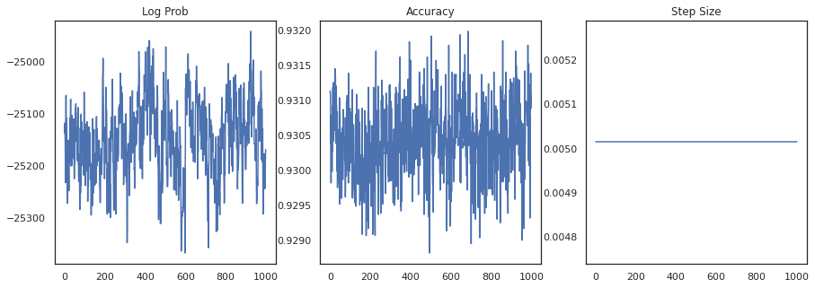
我們正在執行 200,000 個 leapfrog 步驟,每個步驟都會計算整個資料集的梯度。跨 8 個核心分割運算讓我們能夠在大約 95 秒內計算相當於 200,000 個訓練週期的運算,大約每秒 2,100 個週期!
讓我們繪製每個樣本的對數密度和每個樣本的準確度
fig, ax = plt.subplots(1, 3, figsize=(15, 5))
ax[0].plot(trace[0])
ax[0].set_title('Log Prob')
ax[1].plot(trace[1])
ax[1].set_title('Accuracy')
ax[2].plot(trace[2])
ax[2].set_title('Step Size')
plt.show()
如果我們將樣本集成在一起,我們可以計算貝氏模型平均值,以改善我們的效能。
@functools.partial(jax.pmap, axis_name='data', in_axes=(0, None), out_axes=None)
def bayesian_model_average(data, states):
  images, labels = data
  logits = jax.vmap(lambda w, b: images.dot(w) + b)(*states)
  probs = jax.nn.softmax(logits, axis=-1)
  bma_accuracy = (probs.mean(axis=0).argmax(axis=-1) == labels).mean()
  avg_accuracy = (probs.argmax(axis=-1) == labels).mean()
  return lax.pmean(bma_accuracy, axis_name='data'), lax.pmean(avg_accuracy, axis_name='data')

sharded_test_images, sharded_test_labels = shard((test_images, test_labels))
bma_acc, avg_acc = bayesian_model_average((sharded_test_images, sharded_test_labels), states)
print(f'Average Accuracy: {avg_acc}')
print(f'BMA Accuracy: {bma_acc}')
print(f'Accuracy Improvement: {bma_acc - avg_acc}')
Average Accuracy: 0.9188529253005981
BMA Accuracy: 0.9264000058174133
Accuracy Improvement: 0.0075470805168151855
貝氏模型平均值將我們的準確度提高了近 1%!
範例:MovieLens 推薦系統
現在讓我們嘗試使用 MovieLens 推薦資料集進行推論,這是使用者及其對各種電影評分的集合。具體而言,我們可以將 MovieLens 表示為 \(N \times M\) 觀看矩陣 \(W\),其中 \(N\) 是使用者數量,\(M\) 是電影數量;我們預期 \(N > M\)。\(W_{ij}\) 的項目是布林值,表示使用者 \(i\) 是否觀看電影 \(j\)。請注意,MovieLens 提供使用者評分,但為了簡化問題,我們忽略這些評分。
首先,我們將載入資料集。我們將使用包含 100 萬個評分的版本。
movielens = tfds.as_numpy(tfds.load('movielens/1m-ratings', batch_size=-1))
GENRES = ['Action', 'Adventure', 'Animation', 'Children', 'Comedy',
          'Crime', 'Documentary', 'Drama', 'Fantasy', 'Film-Noir',
          'Horror', 'IMAX', 'Musical', 'Mystery', 'Romance', 'Sci-Fi',
          'Thriller', 'Unknown', 'War', 'Western', '(no genres listed)']
Downloading and preparing dataset movielens/1m-ratings/0.1.0 (download: Unknown size, generated: Unknown size, total: Unknown size) to /root/tensorflow_datasets/movielens/1m-ratings/0.1.0...
HBox(children=(FloatProgress(value=1.0, bar_style='info', description='Dl Completed...', max=1.0, style=Progre…
HBox(children=(FloatProgress(value=1.0, bar_style='info', description='Dl Size...', max=1.0, style=ProgressSty…
HBox(children=(FloatProgress(value=1.0, bar_style='info', description='Extraction completed...', max=1.0, styl…

HBox(children=(FloatProgress(value=1.0, bar_style='info', max=1.0), HTML(value='')))
Shuffling and writing examples to /root/tensorflow_datasets/movielens/1m-ratings/0.1.0.incompleteYKA3TG/movielens-train.tfrecord
HBox(children=(FloatProgress(value=0.0, max=1000209.0), HTML(value='')))
Dataset movielens downloaded and prepared to /root/tensorflow_datasets/movielens/1m-ratings/0.1.0. Subsequent calls will reuse this data.
我們將對資料集進行一些前處理,以取得觀看矩陣 \(W\)。
raw_movie_ids = movielens['train']['movie_id']
raw_user_ids = movielens['train']['user_id']
genres = movielens['train']['movie_genres']

movie_ids, movie_labels = pd.factorize(movielens['train']['movie_id'])
user_ids, user_labels = pd.factorize(movielens['train']['user_id'])

num_movies = movie_ids.max() + 1
num_users = user_ids.max() + 1

movie_titles = dict(zip(movielens['train']['movie_id'],
                        movielens['train']['movie_title']))
movie_genres = dict(zip(movielens['train']['movie_id'],
                        genres))
movie_id_to_title = [movie_titles[movie_labels[id]].decode('utf-8')
                     for id in range(num_movies)]
movie_id_to_genre = [GENRES[movie_genres[movie_labels[id]][0]] for id in range(num_movies)]

watch_matrix = np.zeros((num_users, num_movies), bool)
watch_matrix[user_ids, movie_ids] = True
print(watch_matrix.shape)
(6040, 3706)
我們可以為 \(W\) 定義生成模型,使用簡單的機率矩陣分解模型。我們假設潛在的 \(N \times D\) 使用者矩陣 \(U\) 和潛在的 \(M \times D\) 電影矩陣 \(V\),當它們相乘時,會產生觀看矩陣 \(W\) 的 Bernoulli logits。我們也會包含使用者和電影的偏差向量 \(u\) 和 \(v\)。
\[ \begin{align*} U &\sim \mathcal{N}(0, 1) \quad u \sim \mathcal{N}(0, 1)\\ V &\sim \mathcal{N}(0, 1) \quad v \sim \mathcal{N}(0, 1)\\ W_{ij} &\sim \textrm{Bernoulli}\left(\sigma\left(\left(UV^T\right)_{ij} + u_i + v_j\right)\right) \end{align*} \]
這是一個相當大的矩陣;6040 個使用者和 3706 部電影會產生一個包含超過 2200 萬個項目的矩陣。我們應如何處理此模型的分割?嗯,如果我們假設 \(N > M\) (即使用者多於電影),那麼跨使用者軸分割觀看矩陣會很有意義,因此每個裝置都會有一個觀看矩陣區塊,對應於使用者子集。不過,與先前的範例不同,我們也必須分割 \(U\) 矩陣,因為它具有每個使用者的嵌入,因此每個裝置將負責 \(U\) 的分割和 \(W\) 的分割。另一方面,\(V\) 將不會分割,而且會在多個裝置之間同步。
sharded_watch_matrix = shard(watch_matrix)
在我們撰寫 run 之前,我們先快速討論分割本機隨機變數 \(U\) 的其他挑戰。執行 HMC 時,原始 ... 核心將取樣鏈狀態每個元素的動量。先前,只有未分割的隨機變數是該狀態的一部分,而且每個裝置上的動量都相同。當我們現在有一個分割的 \(U\) 時,我們需要在每個裝置上為 \(U\) 取樣不同的動量,同時為 \(V\) 取樣相同的動量。若要完成此操作,我們可以搭配 Sharded 動量分配使用 ...。隨著我們持續將平行運算設為第一類,我們可能會簡化此操作,例如,透過將分割指標新增至 HMC 核心。
def make_run(*,
             axis_name,
             dim=20,
             num_chains=2,
             prior_variance=1.,
             step_size=1e-2,
             num_leapfrog_steps=100,
             num_burnin_steps=1000,
             num_results=500,
             ):
  @functools.partial(jax.pmap, in_axes=(None, 0), axis_name=axis_name)
  @jax.default_matmul_precision('tensorfloat32')
  def run(key, watch_matrix):
    num_users, num_movies = watch_matrix.shape

    Sharded = functools.partial(tfed.Sharded, shard_axis_name=axis_name)

    def prior_fn():
      user_embeddings = yield Root(Sharded(tfd.Sample(tfd.Normal(0., 1.), [num_users, dim]), name='user_embeddings'))
      user_bias = yield Root(Sharded(tfd.Sample(tfd.Normal(0., 1.), [num_users]), name='user_bias'))
      movie_embeddings = yield Root(tfd.Sample(tfd.Normal(0., 1.), [num_movies, dim], name='movie_embeddings'))
      movie_bias = yield Root(tfd.Sample(tfd.Normal(0., 1.), [num_movies], name='movie_bias'))
      return (user_embeddings, user_bias, movie_embeddings, movie_bias)
    prior = tfed.JointDistributionCoroutine(prior_fn)

    def model_fn():
      user_embeddings, user_bias, movie_embeddings, movie_bias = yield from prior_fn()
      logits = (jnp.einsum('...nd,...md->...nm', user_embeddings, movie_embeddings)
                + user_bias[..., :, None] + movie_bias[..., None, :])
      yield Sharded(tfd.Independent(tfd.Bernoulli(logits=logits), 2), name='watch')
    model = tfed.JointDistributionCoroutine(model_fn)

    init_key, sample_key = random.split(key)
    initial_state = prior.sample(seed=init_key, sample_shape=num_chains)

    def target_log_prob(*state):
      return model.log_prob((*state, watch_matrix))

    momentum_distribution = tfed.JointDistributionSequential([
      Sharded(tfd.Independent(tfd.Normal(jnp.zeros([num_chains, num_users, dim]), 1.), 2)),
      Sharded(tfd.Independent(tfd.Normal(jnp.zeros([num_chains, num_users]), 1.), 1)),
      tfd.Independent(tfd.Normal(jnp.zeros([num_chains, num_movies, dim]), 1.), 2),
      tfd.Independent(tfd.Normal(jnp.zeros([num_chains, num_movies]), 1.), 1),
    ])

    # We pass in momentum_distribution here to ensure that the momenta for
    # user_embeddings and user_bias are also sharded
    kernel = tfem.PreconditionedHamiltonianMonteCarlo(target_log_prob, step_size,
                                                      num_leapfrog_steps,
                                                      momentum_distribution=momentum_distribution)

    num_adaptation_steps = int(0.8 * num_burnin_steps)
    kernel = tfm.DualAveragingStepSizeAdaptation(kernel, num_adaptation_steps)

    def trace_fn(state, pkr):
      return {
        'log_prob': target_log_prob(*state),
        'log_accept_ratio': pkr.inner_results.log_accept_ratio,
      }
    return tfm.sample_chain(
        num_results, initial_state,
        kernel=kernel,
        num_burnin_steps=num_burnin_steps,
        trace_fn=trace_fn,
        seed=sample_key)
  return run
我們會再次執行一次,以快取編譯後的 run。
%%time
run = make_run(axis_name='data')
output = run(random.PRNGKey(0), sharded_watch_matrix)
jax.tree.map(lambda x: x.block_until_ready(), output)
CPU times: user 56 s, sys: 1min 24s, total: 2min 20s
Wall time: 3min 35s
現在我們將在沒有編譯額外負荷的情況下再次執行。
%%time
states, trace = run(random.PRNGKey(0), sharded_watch_matrix)
jax.tree.map(lambda x: x.block_until_ready(), trace)
CPU times: user 28.8 s, sys: 1min 16s, total: 1min 44s
Wall time: 3min 1s
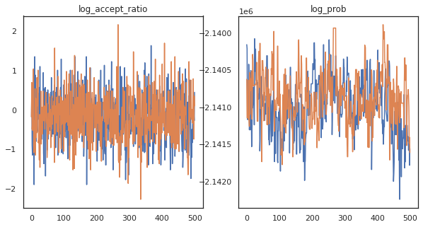
看起來我們在大約 3 分鐘內完成了大約 150,000 個 leapfrog 步驟,因此大約每秒 83 個 leapfrog 步驟!讓我們繪製樣本的接受率和對數密度。
fig, axs = plt.subplots(1, len(trace), figsize=(5 * len(trace), 5))
for ax, (key, val) in zip(axs, trace.items()):
  ax.plot(val[0]) # Indexing into a sharded array, each element is the same
  ax.set_title(key);
現在我們已經從馬可夫鏈取得了一些樣本,讓我們用它們來做一些預測。首先,我們先提取每個組件。請記住,user_embeddings 和 user_bias 是分散在裝置上的,所以我們需要串連我們的 ShardedArray 才能取得所有這些。另一方面,movie_embeddings 和 movie_bias 在每個裝置上都是相同的,所以我們可以從第一個分片中選取值。我們將使用一般的 numpy 將這些值從 TPU 複製回 CPU。
user_embeddings = np.concatenate(np.array(states.user_embeddings, np.float32), axis=2)
user_bias = np.concatenate(np.array(states.user_bias, np.float32), axis=2)
movie_embeddings = np.array(states.movie_embeddings[0], dtype=np.float32)
movie_bias = np.array(states.movie_bias[0], dtype=np.float32)
samples = (user_embeddings, user_bias, movie_embeddings, movie_bias)
print(f'User embeddings: {user_embeddings.shape}')
print(f'User bias: {user_bias.shape}')
print(f'Movie embeddings: {movie_embeddings.shape}')
print(f'Movie bias: {movie_bias.shape}')
User embeddings: (500, 2, 6040, 20)
User bias: (500, 2, 6040)
Movie embeddings: (500, 2, 3706, 20)
Movie bias: (500, 2, 3706)
讓我們嘗試建立一個簡單的推薦系統,利用這些樣本中捕捉到的不確定性。我們先寫一個函數,根據觀看機率對電影進行排名。
@jax.jit
def recommend(sample, user_id):
  user_embeddings, user_bias, movie_embeddings, movie_bias = sample
  movie_logits = (
      jnp.einsum('d,md->m', user_embeddings[user_id], movie_embeddings)
      + user_bias[user_id] + movie_bias)
  return movie_logits.argsort()[::-1]
我們現在可以寫一個函數,遍歷所有樣本,並為每個樣本選取使用者尚未觀看過的排名最高的電影。然後我們可以查看所有樣本中推薦電影的計數。
def get_recommendations(user_id):
  movie_ids = []
  already_watched = set(jnp.arange(num_movies)[watch_matrix[user_id] == 1])
  for i in range(500):
    for j in range(2):
      sample = jax.tree.map(lambda x: x[i, j], samples)
      ranking = recommend(sample, user_id)
      for movie_id in ranking:
        if int(movie_id) not in already_watched:
          movie_ids.append(movie_id)
          break
  return movie_ids

def plot_recommendations(movie_ids, ax=None):
  titles = collections.Counter([movie_id_to_title[i] for i in movie_ids])
  ax = ax or plt.gca()
  names, counts = zip(*sorted(titles.items(), key=lambda x: -x[1]))
  ax.bar(names, counts)
  ax.set_xticklabels(names, rotation=90)
讓我們選取看過最多電影的使用者與看過最少電影的使用者。
user_watch_counts = watch_matrix.sum(axis=1)
user_most = user_watch_counts.argmax()
user_least = user_watch_counts.argmin()
print(user_watch_counts[user_most], user_watch_counts[user_least])
2314 20
我們希望我們的系統對於 user_most 比對 user_least 更有把握,因為我們有更多關於 user_most 更可能觀看哪種類型電影的資訊。
fig, ax = plt.subplots(1, 2, figsize=(20, 10))
most_recommendations = get_recommendations(user_most)
plot_recommendations(most_recommendations, ax=ax[0])
ax[0].set_title('Recommendation for user_most')
least_recommendations = get_recommendations(user_least)
plot_recommendations(least_recommendations, ax=ax[1])
ax[1].set_title('Recommendation for user_least');
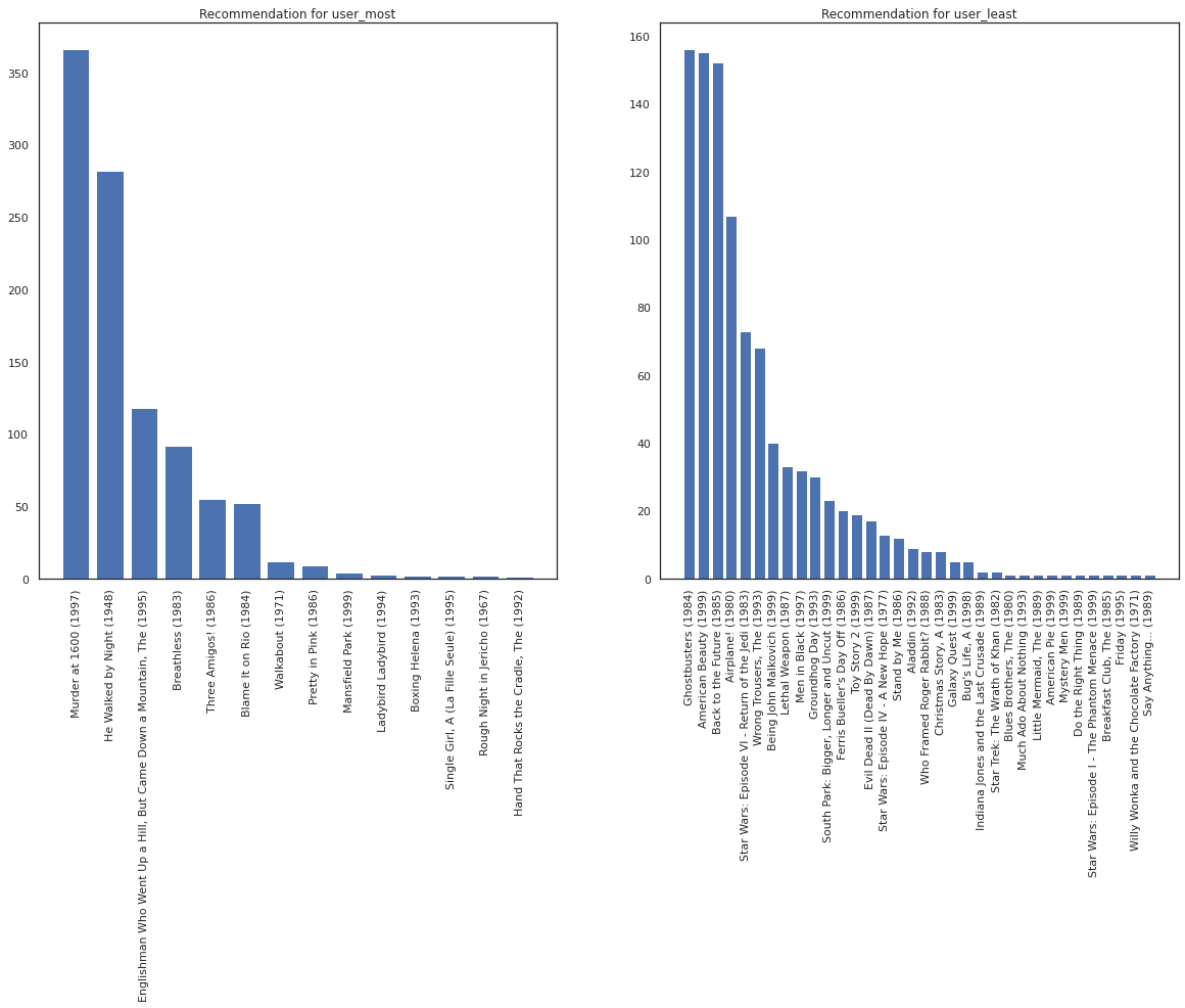
我們看到對於 user_least 的推薦,變異性更大,反映出我們對他們的觀看偏好有更多的不確定性。
我們也可以看看推薦電影的類型。
most_genres = collections.Counter([movie_id_to_genre[i] for i in most_recommendations])
least_genres = collections.Counter([movie_id_to_genre[i] for i in least_recommendations])
fig, ax = plt.subplots(1, 2, figsize=(20, 10))
ax[0].bar(most_genres.keys(), most_genres.values())
ax[0].set_title('Genres recommended for user_most')
ax[1].bar(least_genres.keys(), least_genres.values())
ax[1].set_title('Genres recommended for user_least');
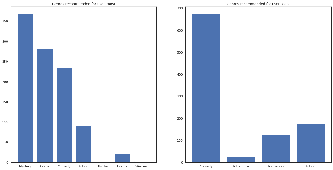
user_most 看過很多電影,並且被推薦了更多小眾類型,如懸疑和犯罪片,而 user_least 沒有看過很多電影,並且被推薦了更多主流電影,這些電影偏向喜劇和動作片。