|
|
|
 在 GitHub 上檢視原始碼 在 GitHub 上檢視原始碼
|
|
這個筆記本重新實作並擴充了 pymc3 文件中的貝氏「變更點分析」範例。
先決條件
import tensorflow.compat.v2 as tf
tf.enable_v2_behavior()
import tensorflow_probability as tfp
tfd = tfp.distributions
tfb = tfp.bijectors
import matplotlib.pyplot as plt
plt.rcParams['figure.figsize'] = (15,8)
%config InlineBackend.figure_format = 'retina'
import numpy as np
import pandas as pd
資料集
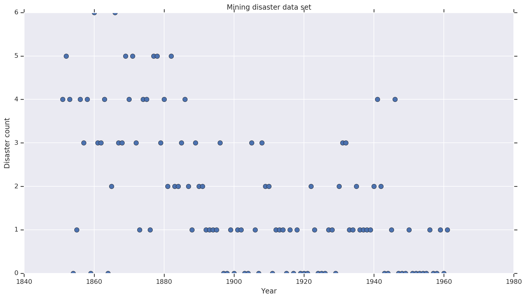
這個資料集取自此處。請注意,另有一個版本的範例在網路上流傳,但該版本缺少資料,在這種情況下,您需要填補遺失值。(否則您的模型將永遠不會離開其初始參數,因為概似函數將未定義。)
disaster_data = np.array([ 4, 5, 4, 0, 1, 4, 3, 4, 0, 6, 3, 3, 4, 0, 2, 6,
                           3, 3, 5, 4, 5, 3, 1, 4, 4, 1, 5, 5, 3, 4, 2, 5,
                           2, 2, 3, 4, 2, 1, 3, 2, 2, 1, 1, 1, 1, 3, 0, 0,
                           1, 0, 1, 1, 0, 0, 3, 1, 0, 3, 2, 2, 0, 1, 1, 1,
                           0, 1, 0, 1, 0, 0, 0, 2, 1, 0, 0, 0, 1, 1, 0, 2,
                           3, 3, 1, 1, 2, 1, 1, 1, 1, 2, 4, 2, 0, 0, 1, 4,
                           0, 0, 0, 1, 0, 0, 0, 0, 0, 1, 0, 0, 1, 0, 1])
years = np.arange(1851, 1962)
plt.plot(years, disaster_data, 'o', markersize=8);
plt.ylabel('Disaster count')
plt.xlabel('Year')
plt.title('Mining disaster data set')
plt.show()
機率模型
此模型假設一個「切換點」(例如安全法規變更的年份),以及在該切換點前後具有恆定 (但可能不同) 比率的卜瓦松分佈災難率。
實際的災難計數是固定的 (已觀察);此模型的任何樣本都需要指定切換點以及「早期」和「晚期」災難率。
原始模型出自 pymc3 文件範例
\[ \begin{align*} (D_t|s,e,l)&\sim \text{Poisson}(r_t), \\ & \,\quad\text{with}\; r_t = \begin{cases}e & \text{if}\; t < s\\l &\text{if}\; t \ge s\end{cases} \\ s&\sim\text{Discrete Uniform}(t_l,\,t_h) \\ e&\sim\text{Exponential}(r_e)\\ l&\sim\text{Exponential}(r_l) \end{align*} \]
然而,平均災難率 \(r_t\) 在切換點 \(s\) 處具有不連續性,這使其不可微分。因此,它沒有為 Hamiltonian Monte Carlo (HMC) 演算法提供梯度訊號,但由於 \(s\) 先驗是連續的,因此 HMC 回退到隨機漫步足以在此範例中找到高機率質量的區域。
作為第二個模型,我們使用介於 *e* 和 *l* 之間的 sigmoid「切換」來修改原始模型,以使過渡可微分,並為切換點 \(s\) 使用連續均勻分佈。(有人可能會認為此模型更符合現實,因為平均比率的「切換」可能會在數年內拉長。) 因此,新模型為
\[ \begin{align*} (D_t|s,e,l)&\sim\text{Poisson}(r_t), \\ & \,\quad \text{with}\; r_t = e + \frac{1}{1+\exp(s-t)}(l-e) \\ s&\sim\text{Uniform}(t_l,\,t_h) \\ e&\sim\text{Exponential}(r_e)\\ l&\sim\text{Exponential}(r_l) \end{align*} \]
在沒有更多資訊的情況下,我們假設 \(r_e = r_l = 1\) 作為先驗的參數。我們將執行這兩個模型並比較它們的推論結果。
def disaster_count_model(disaster_rate_fn):
  disaster_count = tfd.JointDistributionNamed(dict(
    e=tfd.Exponential(rate=1.),
    l=tfd.Exponential(rate=1.),
    s=tfd.Uniform(0., high=len(years)),
    d_t=lambda s, l, e: tfd.Independent(
        tfd.Poisson(rate=disaster_rate_fn(np.arange(len(years)), s, l, e)),
        reinterpreted_batch_ndims=1)
  ))
  return disaster_count

def disaster_rate_switch(ys, s, l, e):
  return tf.where(ys < s, e, l)

def disaster_rate_sigmoid(ys, s, l, e):
  return e + tf.sigmoid(ys - s) * (l - e)

model_switch = disaster_count_model(disaster_rate_switch)
model_sigmoid = disaster_count_model(disaster_rate_sigmoid)
上述程式碼透過 JointDistributionSequential 分佈定義模型。`disaster_rate` 函數會使用 `[0, ..., len(years)-1]` 陣列呼叫,以產生 `len(years)` 個隨機變數的向量 – `switchpoint` 之前的年份是 `early_disaster_rate`,之後的年份是 `late_disaster_rate` (取決於 sigmoid 過渡)。
以下健全性檢查目標對數機率函數是否健全
def target_log_prob_fn(model, s, e, l):
  return model.log_prob(s=s, e=e, l=l, d_t=disaster_data)

models = [model_switch, model_sigmoid]
print([target_log_prob_fn(m, 40., 3., .9).numpy() for m in models])  # Somewhat likely result
print([target_log_prob_fn(m, 60., 1., 5.).numpy() for m in models])  # Rather unlikely result
print([target_log_prob_fn(m, -10., 1., 1.).numpy() for m in models]) # Impossible result
[-176.94559, -176.28717]
[-371.3125, -366.8816]
[-inf, -inf]
使用 HMC 進行貝氏推論
我們定義所需的結果數量和暖機步驟;此程式碼主要仿照 tfp.mcmc.HamiltonianMonteCarlo 的文件。它使用自適應步長 (否則結果會對選擇的步長值非常敏感)。我們使用值 1 作為鏈的初始狀態。
但這並非全貌。如果您回到上面的模型定義,您會注意到某些機率分佈在整個實數線上並未明確定義。因此,我們透過使用 TransformedTransitionKernel 包裝 HMC 核心來限制 HMC 應檢查的空間,TransformedTransitionKernel 指定前向雙射器,以將實數轉換到機率分佈定義的域上 (請參閱以下程式碼中的註解)。
num_results = 10000
num_burnin_steps = 3000

@tf.function(autograph=False, jit_compile=True)
def make_chain(target_log_prob_fn):
   kernel = tfp.mcmc.TransformedTransitionKernel(
       inner_kernel=tfp.mcmc.HamiltonianMonteCarlo(
          target_log_prob_fn=target_log_prob_fn,
          step_size=0.05,
          num_leapfrog_steps=3),
       bijector=[
          # The switchpoint is constrained between zero and len(years).
          # Hence we supply a bijector that maps the real numbers (in a
          # differentiable way) to the interval (0;len(yers))
          tfb.Sigmoid(low=0., high=tf.cast(len(years), dtype=tf.float32)),
          # Early and late disaster rate: The exponential distribution is
          # defined on the positive real numbers
          tfb.Softplus(),
          tfb.Softplus(),
      ])
   kernel = tfp.mcmc.SimpleStepSizeAdaptation(
        inner_kernel=kernel,
        num_adaptation_steps=int(0.8*num_burnin_steps))

   states = tfp.mcmc.sample_chain(
      num_results=num_results,
      num_burnin_steps=num_burnin_steps,
      current_state=[
          # The three latent variables
          tf.ones([], name='init_switchpoint'),
          tf.ones([], name='init_early_disaster_rate'),
          tf.ones([], name='init_late_disaster_rate'),
      ],
      trace_fn=None,
      kernel=kernel)
   return states

switch_samples = [s.numpy() for s in make_chain(
    lambda *args: target_log_prob_fn(model_switch, *args))]
sigmoid_samples = [s.numpy() for s in make_chain(
    lambda *args: target_log_prob_fn(model_sigmoid, *args))]

switchpoint, early_disaster_rate, late_disaster_rate = zip(
    switch_samples, sigmoid_samples)
平行執行兩個模型
將結果視覺化
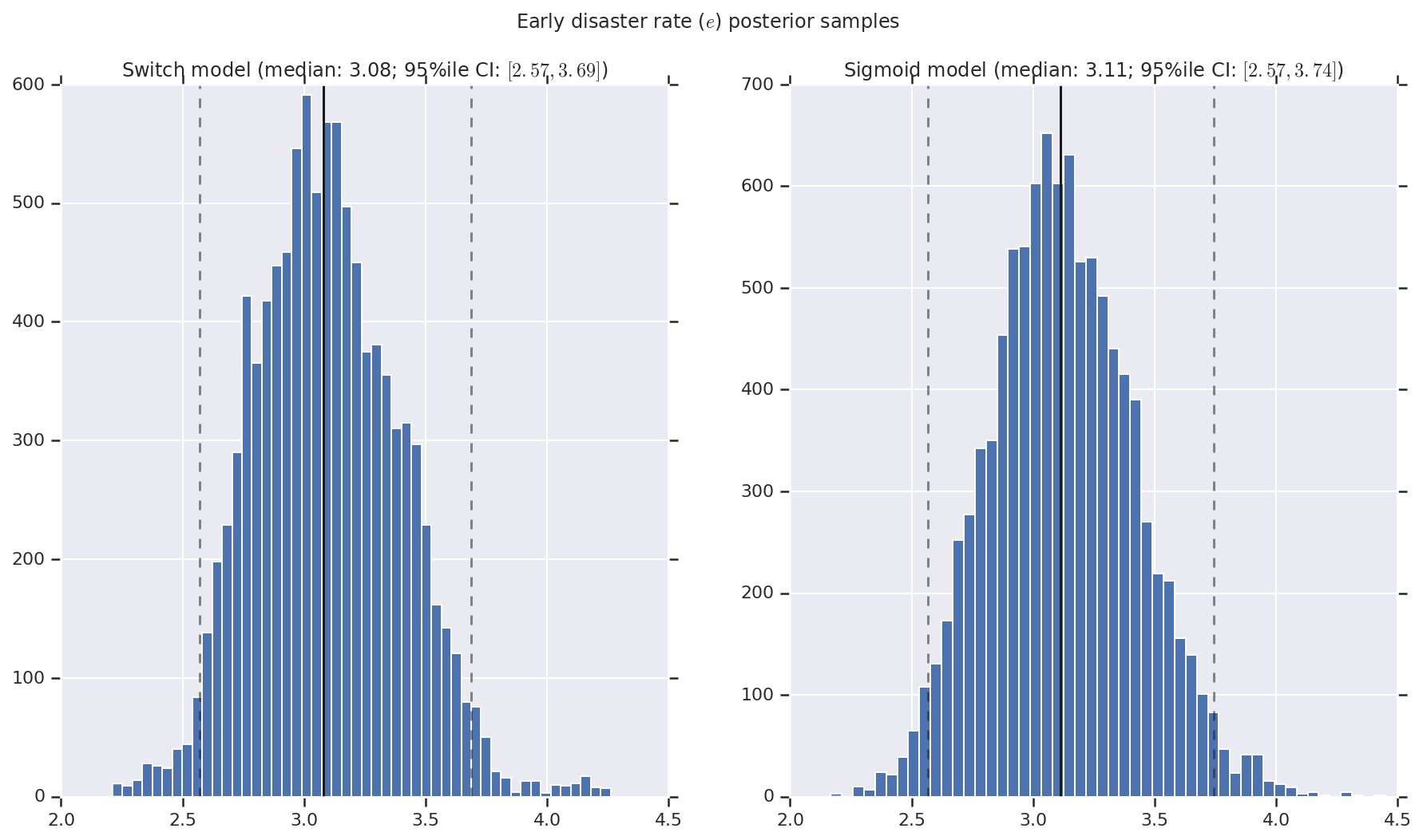
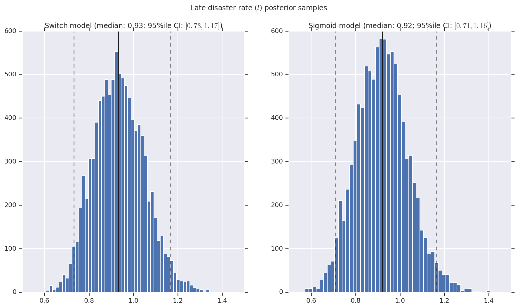
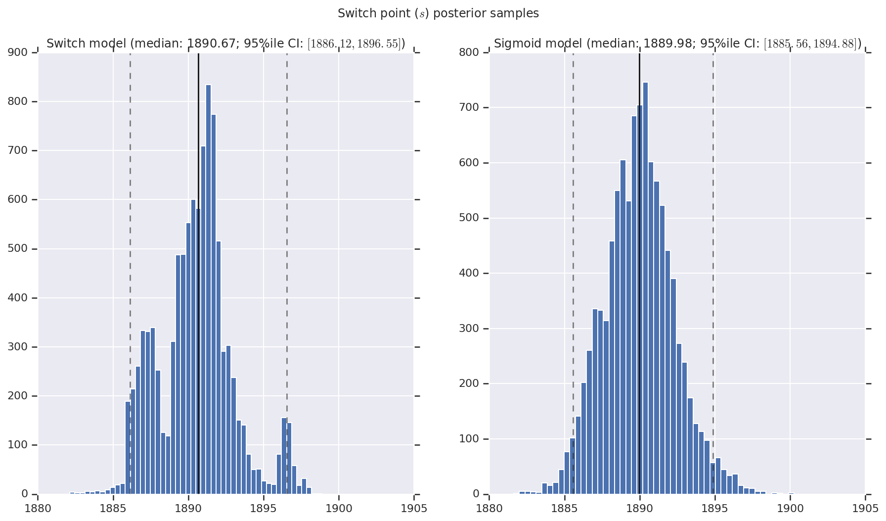
我們將結果視覺化為早期和晚期災難率以及切換點之後驗分佈樣本的直方圖。直方圖覆蓋著代表樣本中位數的實線,以及代表 95% 可信區間邊界的虛線。
def _desc(v):
  return '(median: {}; 95%ile CI: $[{}, {}]$)'.format(
      *np.round(np.percentile(v, [50, 2.5, 97.5]), 2))

for t, v in [
    ('Early disaster rate ($e$) posterior samples', early_disaster_rate),
    ('Late disaster rate ($l$) posterior samples', late_disaster_rate),
    ('Switch point ($s$) posterior samples', years[0] + switchpoint),
]:
  fig, ax = plt.subplots(nrows=1, ncols=2, sharex=True)
  for (m, i) in (('Switch', 0), ('Sigmoid', 1)):
    a = ax[i]
    a.hist(v[i], bins=50)
    a.axvline(x=np.percentile(v[i], 50), color='k')
    a.axvline(x=np.percentile(v[i], 2.5), color='k', ls='dashed', alpha=.5)
    a.axvline(x=np.percentile(v[i], 97.5), color='k', ls='dashed', alpha=.5)
    a.set_title(m + ' model ' + _desc(v[i]))
  fig.suptitle(t)
  plt.show()