
|
|
|
 在 GitHub 上檢視原始碼 在 GitHub 上檢視原始碼
|
|
在這個 Colab 中,我們將探索僅使用 TensorFlow Probability 基本元素,從貝氏高斯混合模型 (BGMM) 後驗分佈中取樣。
模型
對於維度為 \(D\) 的 \(k\in\{1,\ldots, K\}\) 個混合成分,我們希望使用以下貝氏高斯混合模型,對 \(i\in\{1,\ldots,N\}\) 個獨立同分布樣本進行建模
\[\begin{align*} \theta &\sim \text{Dirichlet}(\text{concentration}=\alpha_0)\\ \mu_k &\sim \text{Normal}(\text{loc}=\mu_{0k}, \text{scale}=I_D)\\ T_k &\sim \text{Wishart}(\text{df}=5, \text{scale}=I_D)\\ Z_i &\sim \text{Categorical}(\text{probs}=\theta)\\ Y_i &\sim \text{Normal}(\text{loc}=\mu_{z_i}, \text{scale}=T_{z_i}^{-1/2})\\ \end{align*}\]
請注意,scale 引數都具有 cholesky 語意。我們使用此慣例,因為這是 TF Distributions 的慣例 (其本身使用此慣例部分原因是它在計算上具有優勢)。
我們的目標是從後驗分佈中產生樣本
\[p\left(\theta, \{\mu_k, T_k\}_{k=1}^K \Big| \{y_i\}_{i=1}^N, \alpha_0, \{\mu_{ok}\}_{k=1}^K\right)\]
請注意,\(\{Z_i\}_{i=1}^N\) 不存在 - 我們只對那些不隨 \(N\) 縮放的隨機變數感興趣。(幸運的是,有一個 TF 分配可以處理邊緣化 \(Z_i\)。)
由於計算上難以處理的正規化項,因此無法直接從此分配中取樣。
Metropolis-Hastings 演算法是從難以正規化的分配中取樣的技術。
TensorFlow Probability 提供多種 MCMC 選項,包括多種基於 Metropolis-Hastings 的選項。在本筆記本中,我們將使用漢彌頓蒙地卡羅方法 (tfp.mcmc.HamiltonianMonteCarlo)。HMC 通常是一個不錯的選擇,因為它可以快速收斂、聯合取樣狀態空間 (相對於逐座標),並利用 TF 的優點之一:自動微分。也就是說,從 BGMM 後驗分佈中取樣實際上可能透過其他方法 (例如,Gibb's 取樣) 更好地完成。
%matplotlib inline


import functools

import matplotlib.pyplot as plt; plt.style.use('ggplot')
import numpy as np
import seaborn as sns; sns.set_context('notebook')

import tensorflow.compat.v2 as tf
tf.enable_v2_behavior()
import tensorflow_probability as tfp

tfd = tfp.distributions
tfb = tfp.bijectors

physical_devices = tf.config.experimental.list_physical_devices('GPU')
if len(physical_devices) > 0:
  tf.config.experimental.set_memory_growth(physical_devices[0], True)
在實際建構模型之前,我們需要定義一種新的分配類型。從上面的模型規格中可以清楚看出,我們正在使用逆共變異數矩陣 (即[精確度矩陣](https://en.wikipedia.org/wiki/Precision_(statistics%29)) 參數化 MVN。為了在 TF 中完成此操作,我們需要推出我們的 Bijector。此 Bijector 將使用前向轉換
Y = tf.linalg.triangular_solve((tf.linalg.matrix_transpose(chol_precision_tril), X, adjoint=True) + loc.
而 log_prob 計算只是逆運算,即
X = tf.linalg.matmul(chol_precision_tril, X - loc, adjoint_a=True).
由於 HMC 所需的只是 log_prob,這表示我們避免呼叫 tf.linalg.triangular_solve (就像 tfd.MultivariateNormalTriL 的情況一樣)。這是有利的,因為 tf.linalg.matmul 通常由於更好的快取區域性而更快。
class MVNCholPrecisionTriL(tfd.TransformedDistribution):
  """MVN from loc and (Cholesky) precision matrix."""

  def __init__(self, loc, chol_precision_tril, name=None):
    super(MVNCholPrecisionTriL, self).__init__(
        distribution=tfd.Independent(tfd.Normal(tf.zeros_like(loc),
                                                scale=tf.ones_like(loc)),
                                     reinterpreted_batch_ndims=1),
        bijector=tfb.Chain([
            tfb.Shift(shift=loc),
            tfb.Invert(tfb.ScaleMatvecTriL(scale_tril=chol_precision_tril,
                                           adjoint=True)),
        ]),
        name=name)
tfd.Independent 分配將一個分配的獨立繪圖轉換為具有統計獨立座標的多變數分配。在計算 log_prob 方面,此「中繼分配」表現為事件維度的簡單總和。
另請注意,我們採用了比例矩陣的 adjoint ("轉置")。這是因為如果精確度是逆共變異數,即 \(P=C^{-1}\),且如果 \(C=AA^\top\),則 \(P=BB^{\top}\),其中 \(B=A^{-\top}\)。
由於此分配有點棘手,讓我們快速驗證我們的 MVNCholPrecisionTriL 是否如我們所想的那樣運作。
def compute_sample_stats(d, seed=42, n=int(1e6)):
  x = d.sample(n, seed=seed)
  sample_mean = tf.reduce_mean(x, axis=0, keepdims=True)
  s = x - sample_mean
  sample_cov = tf.linalg.matmul(s, s, adjoint_a=True) / tf.cast(n, s.dtype)
  sample_scale = tf.linalg.cholesky(sample_cov)
  sample_mean = sample_mean[0]
  return [
      sample_mean,
      sample_cov,
      sample_scale,
  ]

dtype = np.float32
true_loc = np.array([1., -1.], dtype=dtype)
true_chol_precision = np.array([[1., 0.],
                                [2., 8.]],
                               dtype=dtype)
true_precision = np.matmul(true_chol_precision, true_chol_precision.T)
true_cov = np.linalg.inv(true_precision)

d = MVNCholPrecisionTriL(
    loc=true_loc,
    chol_precision_tril=true_chol_precision)

[sample_mean, sample_cov, sample_scale] = [
    t.numpy() for t in compute_sample_stats(d)]

print('true mean:', true_loc)
print('sample mean:', sample_mean)
print('true cov:\n', true_cov)
print('sample cov:\n', sample_cov)
true mean: [ 1. -1.]
sample mean: [ 1.0002806 -1.000105 ]
true cov:
 [[ 1.0625   -0.03125 ]
 [-0.03125   0.015625]]
sample cov:
 [[ 1.0641273  -0.03126175]
 [-0.03126175  0.01559312]]
由於樣本平均值和共變異數接近真實平均值和共變異數,因此分配似乎已正確實作。現在,我們將使用 MVNCholPrecisionTriL tfp.distributions.JointDistributionNamed 來指定 BGMM 模型。對於觀測模型,我們將使用 tfd.MixtureSameFamily 自動整合出 \(\{Z_i\}_{i=1}^N\) 繪圖。
dtype = np.float64
dims = 2
components = 3
num_samples = 1000
bgmm = tfd.JointDistributionNamed(dict(
  mix_probs=tfd.Dirichlet(
    concentration=np.ones(components, dtype) / 10.),
  loc=tfd.Independent(
    tfd.Normal(
        loc=np.stack([
            -np.ones(dims, dtype),
            np.zeros(dims, dtype),
            np.ones(dims, dtype),
        ]),
        scale=tf.ones([components, dims], dtype)),
    reinterpreted_batch_ndims=2),
  precision=tfd.Independent(
    tfd.WishartTriL(
        df=5,
        scale_tril=np.stack([np.eye(dims, dtype=dtype)]*components),
        input_output_cholesky=True),
    reinterpreted_batch_ndims=1),
  s=lambda mix_probs, loc, precision: tfd.Sample(tfd.MixtureSameFamily(
      mixture_distribution=tfd.Categorical(probs=mix_probs),
      components_distribution=MVNCholPrecisionTriL(
          loc=loc,
          chol_precision_tril=precision)),
      sample_shape=num_samples)
))
def joint_log_prob(observations, mix_probs, loc, chol_precision):
  """BGMM with priors: loc=Normal, precision=Inverse-Wishart, mix=Dirichlet.

  Args:
    observations: `[n, d]`-shaped `Tensor` representing Bayesian Gaussian
      Mixture model draws. Each sample is a length-`d` vector.
    mix_probs: `[K]`-shaped `Tensor` representing random draw from
      `Dirichlet` prior.
    loc: `[K, d]`-shaped `Tensor` representing the location parameter of the
      `K` components.
    chol_precision: `[K, d, d]`-shaped `Tensor` representing `K` lower
      triangular `cholesky(Precision)` matrices, each being sampled from
      a Wishart distribution.

  Returns:
    log_prob: `Tensor` representing joint log-density over all inputs.
  """
  return bgmm.log_prob(
      mix_probs=mix_probs, loc=loc, precision=chol_precision, s=observations)
產生「訓練」資料
對於此示範,我們將取樣一些隨機資料。
true_loc = np.array([[-2., -2],
                     [0, 0],
                     [2, 2]], dtype)
random = np.random.RandomState(seed=43)

true_hidden_component = random.randint(0, components, num_samples)
observations = (true_loc[true_hidden_component] +
                random.randn(num_samples, dims).astype(dtype))
使用 HMC 的貝氏推論
現在我們已使用 TFD 指定我們的模型並取得一些觀測資料,我們擁有執行 HMC 的所有必要部分。
為此,我們將使用部分應用來「釘住」我們不想取樣的事物。在這種情況下,這表示我們只需要釘住 observations。(超參數已烘焙到先驗分配中,而不是 joint_log_prob 函數簽章的一部分。)
unnormalized_posterior_log_prob = functools.partial(joint_log_prob, observations)
initial_state = [
    tf.fill([components],
            value=np.array(1. / components, dtype),
            name='mix_probs'),
    tf.constant(np.array([[-2., -2],
                          [0, 0],
                          [2, 2]], dtype),
                name='loc'),
    tf.linalg.eye(dims, batch_shape=[components], dtype=dtype, name='chol_precision'),
]
不受約束的表示法
漢彌頓蒙地卡羅方法 (HMC) 需要目標對數機率函數對於其引數而言是可微分的。此外,如果狀態空間不受約束,HMC 可以展現顯著更高的統計效率。
這表示我們在從 BGMM 後驗分佈取樣時必須解決兩個主要問題
- \(\theta\) 表示離散機率向量,即必須滿足 \(\sum_{k=1}^K \theta_k = 1\) 且 \(\theta_k>0\)。
- \(T_k\) 表示逆共變異數矩陣,即必須滿足 \(T_k \succ 0\),即為正定。
為了滿足此要求,我們需要
- 將受約束的變數轉換為不受約束的空間
- 在不受約束的空間中執行 MCMC
- 將不受約束的變數轉換回受約束的空間。
與 MVNCholPrecisionTriL 一樣,我們將使用 Bijector 將隨機變數轉換為不受約束的空間。
Dirichlet透過 softmax 函數轉換為不受約束的空間。我們的精確度隨機變數是正半定矩陣上的分配。為了取消約束這些變數,我們將使用
FillTriangular和TransformDiagonal雙射器。這些將向量轉換為下三角矩陣,並確保對角線為正數。前者很有用,因為它僅允許取樣 \(d(d+1)/2\) 個浮點數,而不是 \(d^2\)。
unconstraining_bijectors = [
    tfb.SoftmaxCentered(),
    tfb.Identity(),
    tfb.Chain([
        tfb.TransformDiagonal(tfb.Softplus()),
        tfb.FillTriangular(),
    ])]
@tf.function(autograph=False)
def sample():
  return tfp.mcmc.sample_chain(
    num_results=2000,
    num_burnin_steps=500,
    current_state=initial_state,
    kernel=tfp.mcmc.SimpleStepSizeAdaptation(
        tfp.mcmc.TransformedTransitionKernel(
            inner_kernel=tfp.mcmc.HamiltonianMonteCarlo(
                target_log_prob_fn=unnormalized_posterior_log_prob,
                 step_size=0.065,
                 num_leapfrog_steps=5),
            bijector=unconstraining_bijectors),
         num_adaptation_steps=400),
    trace_fn=lambda _, pkr: pkr.inner_results.inner_results.is_accepted)

[mix_probs, loc, chol_precision], is_accepted = sample()
我們現在將執行鏈並列印後驗平均值。
acceptance_rate = tf.reduce_mean(tf.cast(is_accepted, dtype=tf.float32)).numpy()
mean_mix_probs = tf.reduce_mean(mix_probs, axis=0).numpy()
mean_loc = tf.reduce_mean(loc, axis=0).numpy()
mean_chol_precision = tf.reduce_mean(chol_precision, axis=0).numpy()
precision = tf.linalg.matmul(chol_precision, chol_precision, transpose_b=True)
print('acceptance_rate:', acceptance_rate)
print('avg mix probs:', mean_mix_probs)
print('avg loc:\n', mean_loc)
print('avg chol(precision):\n', mean_chol_precision)
acceptance_rate: 0.5305
avg mix probs: [0.25248723 0.60729516 0.1402176 ]
avg loc:
 [[-1.96466753 -2.12047249]
 [ 0.27628865  0.22944732]
 [ 2.06461244  2.54216122]]
avg chol(precision):
 [[[ 1.05105032  0.        ]
  [ 0.12699955  1.06553113]]

 [[ 0.76058015  0.        ]
  [-0.50332767  0.77947431]]

 [[ 1.22770457  0.        ]
  [ 0.70670027  1.50914164]]]
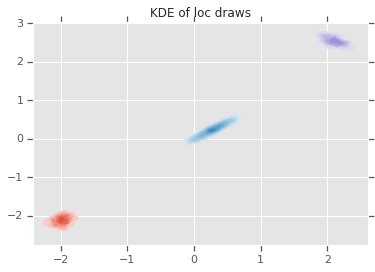
loc_ = loc.numpy()
ax = sns.kdeplot(loc_[:,0,0], loc_[:,0,1], shade=True, shade_lowest=False)
ax = sns.kdeplot(loc_[:,1,0], loc_[:,1,1], shade=True, shade_lowest=False)
ax = sns.kdeplot(loc_[:,2,0], loc_[:,2,1], shade=True, shade_lowest=False)
plt.title('KDE of loc draws');
結論
這個簡單的 Colab 示範了如何使用 TensorFlow Probability 基本元素來建構階層式貝氏混合模型。