|
|
|
 在 GitHub 上檢視原始碼 在 GitHub 上檢視原始碼
|
|
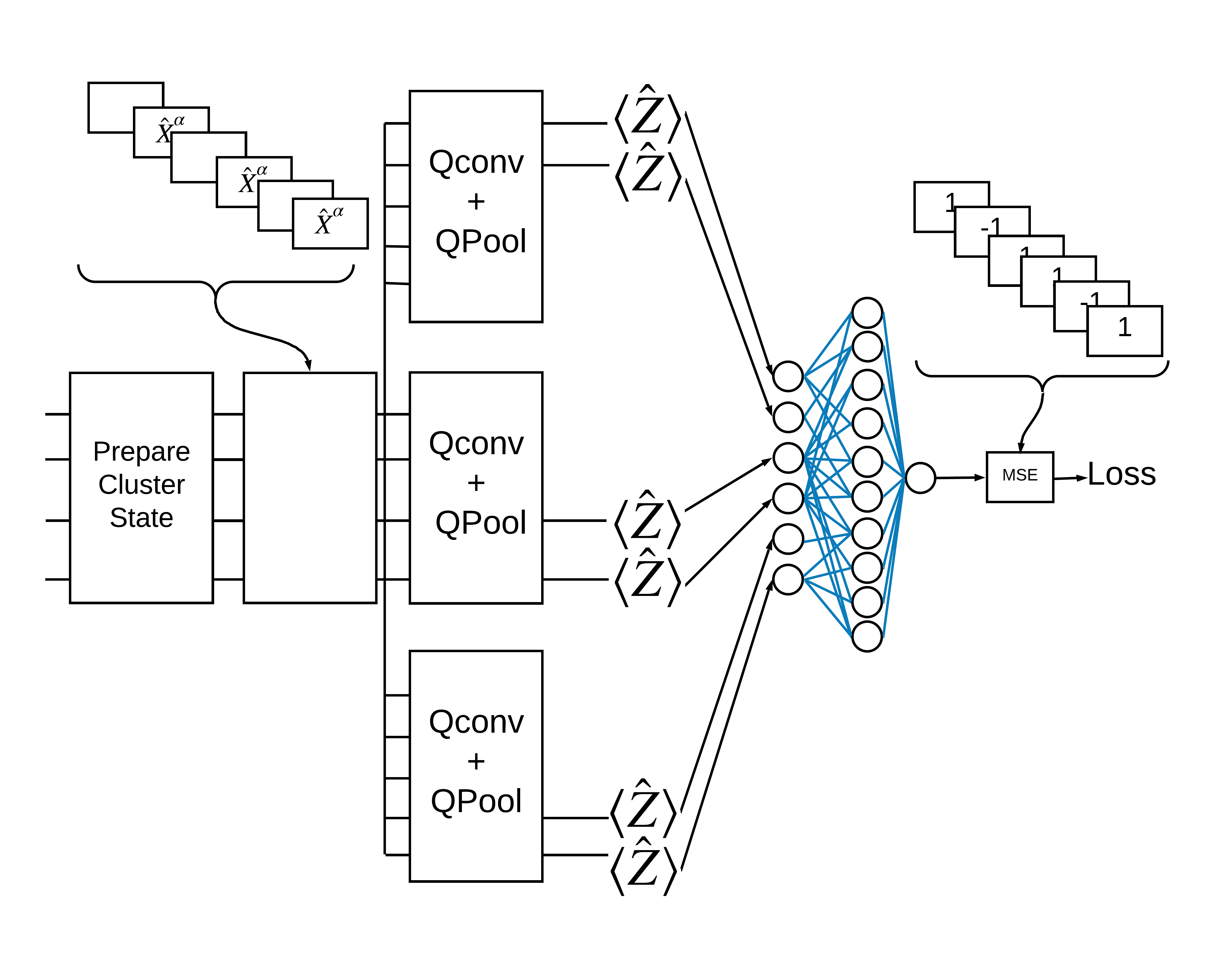
本教學課程實作簡化的量子卷積神經網路 (QCNN),這是一種提議的量子類比,對應於也具有平移不變性的傳統卷積神經網路。
本範例示範如何偵測量子資料來源的特定屬性,例如量子感測器或裝置的複雜模擬。量子資料來源是叢集狀態,可能具有或不具有激發 - 這將是 QCNN 將學習偵測的目標 (本文中使用的資料集是 SPT 相位分類)。
設定
pip install tensorflow==2.15.0
安裝 TensorFlow Quantum
pip install tensorflow-quantum==0.7.3
# Update package resources to account for version changes.
import importlib, pkg_resources
importlib.reload(pkg_resources)
/tmpfs/tmp/ipykernel_26901/1875984233.py:2: DeprecationWarning: pkg_resources is deprecated as an API. See https://setuptools.pypa.io/en/latest/pkg_resources.html
  import importlib, pkg_resources
<module 'pkg_resources' from '/tmpfs/src/tf_docs_env/lib/python3.9/site-packages/pkg_resources/__init__.py'>
現在匯入 TensorFlow 和模組依附元件
import tensorflow as tf
import tensorflow_quantum as tfq

import cirq
import sympy
import numpy as np

# visualization tools
%matplotlib inline
import matplotlib.pyplot as plt
from cirq.contrib.svg import SVGCircuit
2024-05-18 11:45:09.533738: E external/local_xla/xla/stream_executor/cuda/cuda_dnn.cc:9261] Unable to register cuDNN factory: Attempting to register factory for plugin cuDNN when one has already been registered
2024-05-18 11:45:09.533782: E external/local_xla/xla/stream_executor/cuda/cuda_fft.cc:607] Unable to register cuFFT factory: Attempting to register factory for plugin cuFFT when one has already been registered
2024-05-18 11:45:09.535253: E external/local_xla/xla/stream_executor/cuda/cuda_blas.cc:1515] Unable to register cuBLAS factory: Attempting to register factory for plugin cuBLAS when one has already been registered
2024-05-18 11:45:12.910225: E external/local_xla/xla/stream_executor/cuda/cuda_driver.cc:274] failed call to cuInit: CUDA_ERROR_NO_DEVICE: no CUDA-capable device is detected
1. 建構 QCNN
1.1 在 TensorFlow 圖表中組裝電路
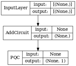
TensorFlow Quantum (TFQ) 提供專為圖表內電路建構而設計的層級類別。其中一個範例是繼承自 tf.keras.Layer 的 tfq.layers.AddCircuit 層級。此層級可以前置或附加到輸入批次的電路,如下圖所示。
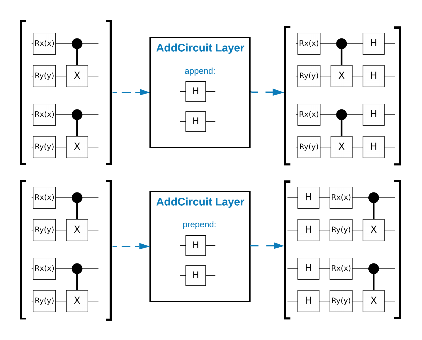
以下程式碼片段使用此層級
qubit = cirq.GridQubit(0, 0)

# Define some circuits.
circuit1 = cirq.Circuit(cirq.X(qubit))
circuit2 = cirq.Circuit(cirq.H(qubit))

# Convert to a tensor.
input_circuit_tensor = tfq.convert_to_tensor([circuit1, circuit2])

# Define a circuit that we want to append
y_circuit = cirq.Circuit(cirq.Y(qubit))

# Instantiate our layer
y_appender = tfq.layers.AddCircuit()

# Run our circuit tensor through the layer and save the output.
output_circuit_tensor = y_appender(input_circuit_tensor, append=y_circuit)
檢查輸入張量
print(tfq.from_tensor(input_circuit_tensor))
[cirq.Circuit([
     cirq.Moment(
         cirq.X(cirq.GridQubit(0, 0)),
     ),
 ])
 cirq.Circuit([
     cirq.Moment(
         cirq.H(cirq.GridQubit(0, 0)),
     ),
 ])                                   ]
並檢查輸出張量
print(tfq.from_tensor(output_circuit_tensor))
[cirq.Circuit([
     cirq.Moment(
         cirq.X(cirq.GridQubit(0, 0)),
     ),
     cirq.Moment(
         cirq.Y(cirq.GridQubit(0, 0)),
     ),
 ])
 cirq.Circuit([
     cirq.Moment(
         cirq.H(cirq.GridQubit(0, 0)),
     ),
     cirq.Moment(
         cirq.Y(cirq.GridQubit(0, 0)),
     ),
 ])                                   ]
雖然可以不使用 tfq.layers.AddCircuit 來執行以下範例,但這是瞭解如何將複雜功能嵌入 TensorFlow 計算圖表的好機會。
1.2 問題總覽
您將準備叢集狀態,並訓練量子分類器來偵測它是否「激發」。叢集狀態高度糾纏,但對於傳統電腦而言不一定困難。為了清楚起見,這是一個比本文中使用的資料集更簡單的資料集。
對於此分類任務,您將實作深度 MERA 類型的 QCNN 架構,因為
- 與 QCNN 類似,環上的叢集狀態具有平移不變性。
- 叢集狀態高度糾纏。
此架構應能有效減少糾纏,透過讀取單一量子位元來獲得分類。
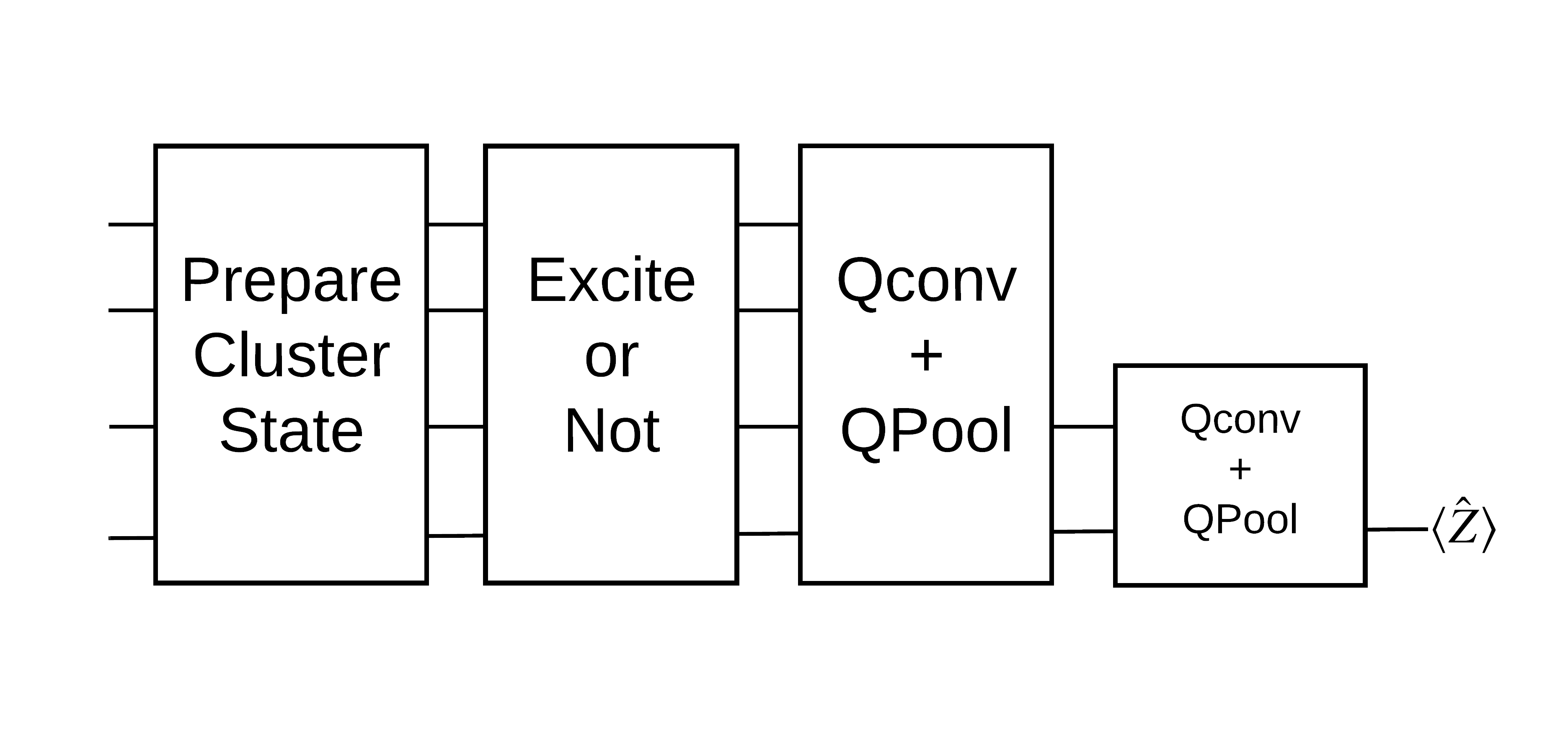
「激發」叢集狀態定義為已將 cirq.rx 閘套用至其任何量子位元的叢集狀態。Qconv 和 QPool 將在本教學課程稍後討論。
1.3 TensorFlow 的建構區塊
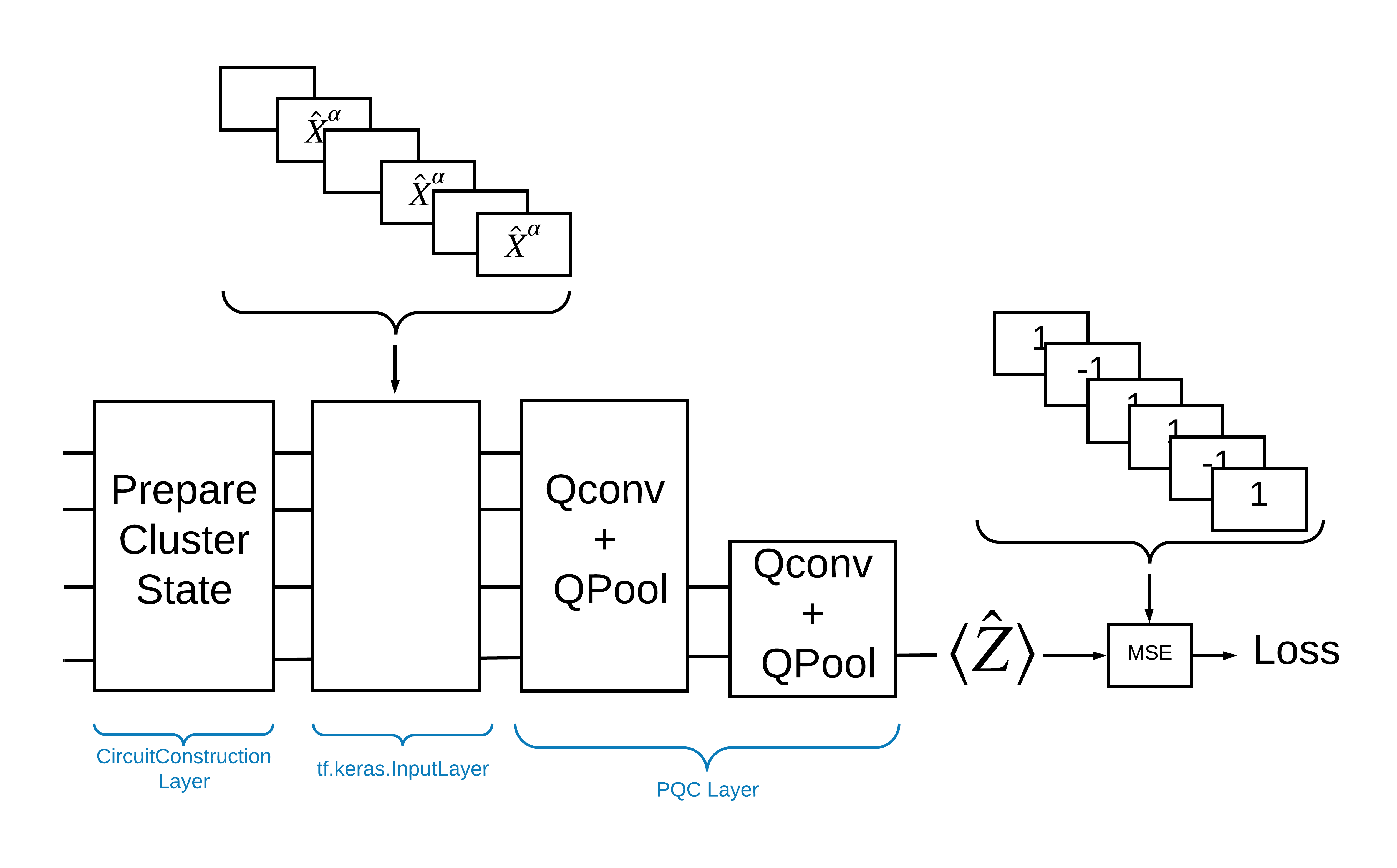
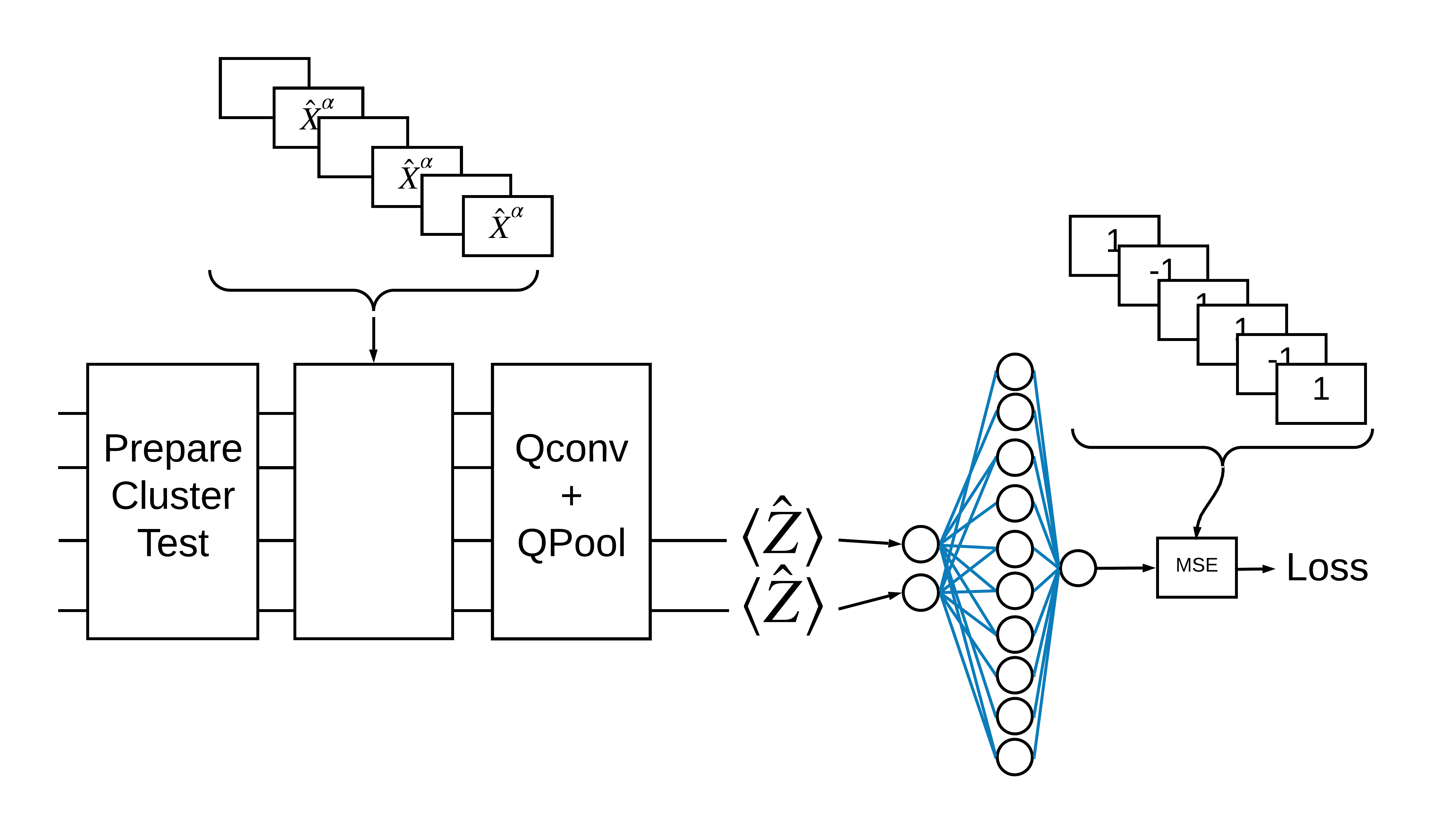
使用 TensorFlow Quantum 解決此問題的一種方法是實作以下項目
- 模型的輸入是電路張量 - 空電路或特定量子位元上的 X 閘,表示激發。
- 模型的其餘量子元件使用
tfq.layers.AddCircuit層級建構。 - 為了進行推論,使用了
tfq.layers.PQC層級。這會讀取 \(\langle \hat{Z} \rangle\),並將其與激發狀態的標籤 1 或非激發狀態的標籤 -1 進行比較。
1.4 資料
在建構模型之前,您可以產生資料。在本例中,它將是叢集狀態的激發 (原始論文使用了更複雜的資料集)。激發以 cirq.rx 閘表示。足夠大的旋轉被視為激發並標記為 1,而旋轉不夠大則標記為 -1 並視為非激發。
def generate_data(qubits):
    """Generate training and testing data."""
    n_rounds = 20  # Produces n_rounds * n_qubits datapoints.
    excitations = []
    labels = []
    for n in range(n_rounds):
        for bit in qubits:
            rng = np.random.uniform(-np.pi, np.pi)
            excitations.append(cirq.Circuit(cirq.rx(rng)(bit)))
            labels.append(1 if (-np.pi / 2) <= rng <= (np.pi / 2) else -1)

    split_ind = int(len(excitations) * 0.7)
    train_excitations = excitations[:split_ind]
    test_excitations = excitations[split_ind:]

    train_labels = labels[:split_ind]
    test_labels = labels[split_ind:]

    return tfq.convert_to_tensor(train_excitations), np.array(train_labels), \
        tfq.convert_to_tensor(test_excitations), np.array(test_labels)
您可以看到,就像使用一般機器學習一樣,您建立訓練和測試集以用於基準化模型。您可以使用以下程式碼快速查看一些資料點
sample_points, sample_labels, _, __ = generate_data(cirq.GridQubit.rect(1, 4))
print('Input:', tfq.from_tensor(sample_points)[0], 'Output:', sample_labels[0])
print('Input:', tfq.from_tensor(sample_points)[1], 'Output:', sample_labels[1])
Input: (0, 0): ───X^0.701─── Output: -1
Input: (0, 1): ───X^-0.136─── Output: 1
1.5 定義層級
現在在 TensorFlow 中定義上圖中顯示的層級。
1.5.1 叢集狀態
第一步是使用 Google 提供的量子電路程式設計架構 Cirq 定義 叢集狀態。由於這是模型的靜態部分,因此使用 tfq.layers.AddCircuit 功能嵌入它。
def cluster_state_circuit(bits):
    """Return a cluster state on the qubits in `bits`."""
    circuit = cirq.Circuit()
    circuit.append(cirq.H.on_each(bits))
    for this_bit, next_bit in zip(bits, bits[1:] + [bits[0]]):
        circuit.append(cirq.CZ(this_bit, next_bit))
    return circuit
顯示 cirq.GridQubit 矩形的叢集狀態電路
SVGCircuit(cluster_state_circuit(cirq.GridQubit.rect(1, 4)))
findfont: Font family 'Arial' not found.
findfont: Font family 'Arial' not found.
findfont: Font family 'Arial' not found.
findfont: Font family 'Arial' not found.
findfont: Font family 'Arial' not found.
findfont: Font family 'Arial' not found.
findfont: Font family 'Arial' not found.
findfont: Font family 'Arial' not found.
findfont: Font family 'Arial' not found.
findfont: Font family 'Arial' not found.
findfont: Font family 'Arial' not found.
findfont: Font family 'Arial' not found.
findfont: Font family 'Arial' not found.
findfont: Font family 'Arial' not found.
findfont: Font family 'Arial' not found.
findfont: Font family 'Arial' not found.

1.5.2 QCNN 層級
使用 Cong 和 Lukin QCNN 論文中定義的層級,構成模型。有一些先決條件
- 來自 Tucci 論文的單一量子位元和雙量子位元參數化么正矩陣。
- 一般參數化雙量子位元集區運算。
def one_qubit_unitary(bit, symbols):
    """Make a Cirq circuit enacting a rotation of the bloch sphere about the X,
    Y and Z axis, that depends on the values in `symbols`.
    """
    return cirq.Circuit(
        cirq.X(bit)**symbols[0],
        cirq.Y(bit)**symbols[1],
        cirq.Z(bit)**symbols[2])


def two_qubit_unitary(bits, symbols):
    """Make a Cirq circuit that creates an arbitrary two qubit unitary."""
    circuit = cirq.Circuit()
    circuit += one_qubit_unitary(bits[0], symbols[0:3])
    circuit += one_qubit_unitary(bits[1], symbols[3:6])
    circuit += [cirq.ZZ(*bits)**symbols[6]]
    circuit += [cirq.YY(*bits)**symbols[7]]
    circuit += [cirq.XX(*bits)**symbols[8]]
    circuit += one_qubit_unitary(bits[0], symbols[9:12])
    circuit += one_qubit_unitary(bits[1], symbols[12:])
    return circuit


def two_qubit_pool(source_qubit, sink_qubit, symbols):
    """Make a Cirq circuit to do a parameterized 'pooling' operation, which
    attempts to reduce entanglement down from two qubits to just one."""
    pool_circuit = cirq.Circuit()
    sink_basis_selector = one_qubit_unitary(sink_qubit, symbols[0:3])
    source_basis_selector = one_qubit_unitary(source_qubit, symbols[3:6])
    pool_circuit.append(sink_basis_selector)
    pool_circuit.append(source_basis_selector)
    pool_circuit.append(cirq.CNOT(source_qubit, sink_qubit))
    pool_circuit.append(sink_basis_selector**-1)
    return pool_circuit
若要查看您建立的內容,請列印單一量子位元么正電路
SVGCircuit(one_qubit_unitary(cirq.GridQubit(0, 0), sympy.symbols('x0:3')))
findfont: Font family 'Arial' not found.
findfont: Font family 'Arial' not found.
findfont: Font family 'Arial' not found.
findfont: Font family 'Arial' not found.

以及雙量子位元么正電路
SVGCircuit(two_qubit_unitary(cirq.GridQubit.rect(1, 2), sympy.symbols('x0:15')))
findfont: Font family 'Arial' not found.
findfont: Font family 'Arial' not found.
findfont: Font family 'Arial' not found.
findfont: Font family 'Arial' not found.
findfont: Font family 'Arial' not found.
findfont: Font family 'Arial' not found.
findfont: Font family 'Arial' not found.
findfont: Font family 'Arial' not found.
findfont: Font family 'Arial' not found.
findfont: Font family 'Arial' not found.
findfont: Font family 'Arial' not found.
findfont: Font family 'Arial' not found.
findfont: Font family 'Arial' not found.
findfont: Font family 'Arial' not found.
findfont: Font family 'Arial' not found.
findfont: Font family 'Arial' not found.
findfont: Font family 'Arial' not found.
findfont: Font family 'Arial' not found.
findfont: Font family 'Arial' not found.
findfont: Font family 'Arial' not found.

以及雙量子位元集區電路
SVGCircuit(two_qubit_pool(*cirq.GridQubit.rect(1, 2), sympy.symbols('x0:6')))
findfont: Font family 'Arial' not found.
findfont: Font family 'Arial' not found.
findfont: Font family 'Arial' not found.
findfont: Font family 'Arial' not found.
findfont: Font family 'Arial' not found.
findfont: Font family 'Arial' not found.
findfont: Font family 'Arial' not found.
findfont: Font family 'Arial' not found.
findfont: Font family 'Arial' not found.
findfont: Font family 'Arial' not found.
findfont: Font family 'Arial' not found.
findfont: Font family 'Arial' not found.
findfont: Font family 'Arial' not found.

1.5.2.1 量子卷積
如同 Cong 和 Lukin 論文中,將 1D 量子卷積定義為將雙量子位元參數化么正套用至每個相鄰量子位元對,步幅為一。
def quantum_conv_circuit(bits, symbols):
    """Quantum Convolution Layer following the above diagram.
    Return a Cirq circuit with the cascade of `two_qubit_unitary` applied
    to all pairs of qubits in `bits` as in the diagram above.
    """
    circuit = cirq.Circuit()
    for first, second in zip(bits[0::2], bits[1::2]):
        circuit += two_qubit_unitary([first, second], symbols)
    for first, second in zip(bits[1::2], bits[2::2] + [bits[0]]):
        circuit += two_qubit_unitary([first, second], symbols)
    return circuit
顯示 (非常水平) 電路
SVGCircuit(
    quantum_conv_circuit(cirq.GridQubit.rect(1, 8), sympy.symbols('x0:15')))
findfont: Font family 'Arial' not found.
findfont: Font family 'Arial' not found.
findfont: Font family 'Arial' not found.
findfont: Font family 'Arial' not found.
findfont: Font family 'Arial' not found.
findfont: Font family 'Arial' not found.
findfont: Font family 'Arial' not found.
findfont: Font family 'Arial' not found.
findfont: Font family 'Arial' not found.
findfont: Font family 'Arial' not found.
findfont: Font family 'Arial' not found.
findfont: Font family 'Arial' not found.
findfont: Font family 'Arial' not found.
findfont: Font family 'Arial' not found.
findfont: Font family 'Arial' not found.
findfont: Font family 'Arial' not found.
findfont: Font family 'Arial' not found.
findfont: Font family 'Arial' not found.
findfont: Font family 'Arial' not found.
findfont: Font family 'Arial' not found.
findfont: Font family 'Arial' not found.
findfont: Font family 'Arial' not found.
findfont: Font family 'Arial' not found.
findfont: Font family 'Arial' not found.
findfont: Font family 'Arial' not found.
findfont: Font family 'Arial' not found.
findfont: Font family 'Arial' not found.
findfont: Font family 'Arial' not found.
findfont: Font family 'Arial' not found.
findfont: Font family 'Arial' not found.
findfont: Font family 'Arial' not found.
findfont: Font family 'Arial' not found.
findfont: Font family 'Arial' not found.
findfont: Font family 'Arial' not found.
findfont: Font family 'Arial' not found.
findfont: Font family 'Arial' not found.
findfont: Font family 'Arial' not found.
findfont: Font family 'Arial' not found.
findfont: Font family 'Arial' not found.
findfont: Font family 'Arial' not found.
findfont: Font family 'Arial' not found.
findfont: Font family 'Arial' not found.
findfont: Font family 'Arial' not found.
findfont: Font family 'Arial' not found.
findfont: Font family 'Arial' not found.
findfont: Font family 'Arial' not found.
findfont: Font family 'Arial' not found.
findfont: Font family 'Arial' not found.
findfont: Font family 'Arial' not found.
findfont: Font family 'Arial' not found.
findfont: Font family 'Arial' not found.
findfont: Font family 'Arial' not found.
findfont: Font family 'Arial' not found.
findfont: Font family 'Arial' not found.
findfont: Font family 'Arial' not found.
findfont: Font family 'Arial' not found.
findfont: Font family 'Arial' not found.
findfont: Font family 'Arial' not found.
findfont: Font family 'Arial' not found.
findfont: Font family 'Arial' not found.
findfont: Font family 'Arial' not found.
findfont: Font family 'Arial' not found.
findfont: Font family 'Arial' not found.
findfont: Font family 'Arial' not found.
findfont: Font family 'Arial' not found.
findfont: Font family 'Arial' not found.
findfont: Font family 'Arial' not found.
findfont: Font family 'Arial' not found.
findfont: Font family 'Arial' not found.
findfont: Font family 'Arial' not found.
findfont: Font family 'Arial' not found.
findfont: Font family 'Arial' not found.
findfont: Font family 'Arial' not found.
findfont: Font family 'Arial' not found.
findfont: Font family 'Arial' not found.
findfont: Font family 'Arial' not found.
findfont: Font family 'Arial' not found.
findfont: Font family 'Arial' not found.
findfont: Font family 'Arial' not found.
findfont: Font family 'Arial' not found.
findfont: Font family 'Arial' not found.
findfont: Font family 'Arial' not found.
findfont: Font family 'Arial' not found.
findfont: Font family 'Arial' not found.
findfont: Font family 'Arial' not found.
findfont: Font family 'Arial' not found.
findfont: Font family 'Arial' not found.
findfont: Font family 'Arial' not found.
findfont: Font family 'Arial' not found.
findfont: Font family 'Arial' not found.
findfont: Font family 'Arial' not found.
findfont: Font family 'Arial' not found.
findfont: Font family 'Arial' not found.
findfont: Font family 'Arial' not found.
findfont: Font family 'Arial' not found.
findfont: Font family 'Arial' not found.
findfont: Font family 'Arial' not found.
findfont: Font family 'Arial' not found.
findfont: Font family 'Arial' not found.
findfont: Font family 'Arial' not found.
findfont: Font family 'Arial' not found.
findfont: Font family 'Arial' not found.
findfont: Font family 'Arial' not found.
findfont: Font family 'Arial' not found.
findfont: Font family 'Arial' not found.
findfont: Font family 'Arial' not found.
findfont: Font family 'Arial' not found.
findfont: Font family 'Arial' not found.
findfont: Font family 'Arial' not found.
findfont: Font family 'Arial' not found.
findfont: Font family 'Arial' not found.
findfont: Font family 'Arial' not found.
findfont: Font family 'Arial' not found.
findfont: Font family 'Arial' not found.
findfont: Font family 'Arial' not found.
findfont: Font family 'Arial' not found.
findfont: Font family 'Arial' not found.
findfont: Font family 'Arial' not found.
findfont: Font family 'Arial' not found.
findfont: Font family 'Arial' not found.
findfont: Font family 'Arial' not found.
findfont: Font family 'Arial' not found.
findfont: Font family 'Arial' not found.
findfont: Font family 'Arial' not found.
findfont: Font family 'Arial' not found.
findfont: Font family 'Arial' not found.
findfont: Font family 'Arial' not found.
findfont: Font family 'Arial' not found.
findfont: Font family 'Arial' not found.
findfont: Font family 'Arial' not found.
findfont: Font family 'Arial' not found.
findfont: Font family 'Arial' not found.
findfont: Font family 'Arial' not found.
findfont: Font family 'Arial' not found.
findfont: Font family 'Arial' not found.
findfont: Font family 'Arial' not found.
findfont: Font family 'Arial' not found.
findfont: Font family 'Arial' not found.
findfont: Font family 'Arial' not found.
findfont: Font family 'Arial' not found.
findfont: Font family 'Arial' not found.
findfont: Font family 'Arial' not found.
findfont: Font family 'Arial' not found.
findfont: Font family 'Arial' not found.
findfont: Font family 'Arial' not found.
findfont: Font family 'Arial' not found.
findfont: Font family 'Arial' not found.
findfont: Font family 'Arial' not found.
findfont: Font family 'Arial' not found.
findfont: Font family 'Arial' not found.
findfont: Font family 'Arial' not found.
findfont: Font family 'Arial' not found.

1.5.2.2 量子集區化
量子集區化層級使用上述定義的雙量子位元集區,從 \(N\) 個量子位元集區化到 \(\frac{N}{2}\) 個量子位元。
def quantum_pool_circuit(source_bits, sink_bits, symbols):
    """A layer that specifies a quantum pooling operation.
    A Quantum pool tries to learn to pool the relevant information from two
    qubits onto 1.
    """
    circuit = cirq.Circuit()
    for source, sink in zip(source_bits, sink_bits):
        circuit += two_qubit_pool(source, sink, symbols)
    return circuit
檢查集區化元件電路
test_bits = cirq.GridQubit.rect(1, 8)

SVGCircuit(
    quantum_pool_circuit(test_bits[:4], test_bits[4:], sympy.symbols('x0:6')))
findfont: Font family 'Arial' not found.
findfont: Font family 'Arial' not found.
findfont: Font family 'Arial' not found.
findfont: Font family 'Arial' not found.
findfont: Font family 'Arial' not found.
findfont: Font family 'Arial' not found.
findfont: Font family 'Arial' not found.
findfont: Font family 'Arial' not found.
findfont: Font family 'Arial' not found.
findfont: Font family 'Arial' not found.
findfont: Font family 'Arial' not found.
findfont: Font family 'Arial' not found.
findfont: Font family 'Arial' not found.
findfont: Font family 'Arial' not found.
findfont: Font family 'Arial' not found.
findfont: Font family 'Arial' not found.
findfont: Font family 'Arial' not found.
findfont: Font family 'Arial' not found.
findfont: Font family 'Arial' not found.
findfont: Font family 'Arial' not found.
findfont: Font family 'Arial' not found.
findfont: Font family 'Arial' not found.
findfont: Font family 'Arial' not found.
findfont: Font family 'Arial' not found.
findfont: Font family 'Arial' not found.
findfont: Font family 'Arial' not found.
findfont: Font family 'Arial' not found.
findfont: Font family 'Arial' not found.
findfont: Font family 'Arial' not found.
findfont: Font family 'Arial' not found.
findfont: Font family 'Arial' not found.
findfont: Font family 'Arial' not found.
findfont: Font family 'Arial' not found.
findfont: Font family 'Arial' not found.
findfont: Font family 'Arial' not found.
findfont: Font family 'Arial' not found.
findfont: Font family 'Arial' not found.
findfont: Font family 'Arial' not found.
findfont: Font family 'Arial' not found.
findfont: Font family 'Arial' not found.
findfont: Font family 'Arial' not found.
findfont: Font family 'Arial' not found.
findfont: Font family 'Arial' not found.
findfont: Font family 'Arial' not found.
findfont: Font family 'Arial' not found.
findfont: Font family 'Arial' not found.
findfont: Font family 'Arial' not found.
findfont: Font family 'Arial' not found.
findfont: Font family 'Arial' not found.
findfont: Font family 'Arial' not found.
findfont: Font family 'Arial' not found.
findfont: Font family 'Arial' not found.

1.6 模型定義
現在使用定義的層級來建構純粹的量子 CNN。從八個量子位元開始,集區化到一個,然後測量 \(\langle \hat{Z} \rangle\)。
def create_model_circuit(qubits):
    """Create sequence of alternating convolution and pooling operators
    which gradually shrink over time."""
    model_circuit = cirq.Circuit()
    symbols = sympy.symbols('qconv0:63')
    # Cirq uses sympy.Symbols to map learnable variables. TensorFlow Quantum
    # scans incoming circuits and replaces these with TensorFlow variables.
    model_circuit += quantum_conv_circuit(qubits, symbols[0:15])
    model_circuit += quantum_pool_circuit(qubits[:4], qubits[4:],
                                          symbols[15:21])
    model_circuit += quantum_conv_circuit(qubits[4:], symbols[21:36])
    model_circuit += quantum_pool_circuit(qubits[4:6], qubits[6:],
                                          symbols[36:42])
    model_circuit += quantum_conv_circuit(qubits[6:], symbols[42:57])
    model_circuit += quantum_pool_circuit([qubits[6]], [qubits[7]],
                                          symbols[57:63])
    return model_circuit


# Create our qubits and readout operators in Cirq.
cluster_state_bits = cirq.GridQubit.rect(1, 8)
readout_operators = cirq.Z(cluster_state_bits[-1])

# Build a sequential model enacting the logic in 1.3 of this notebook.
# Here you are making the static cluster state prep as a part of the AddCircuit and the
# "quantum datapoints" are coming in the form of excitation
excitation_input = tf.keras.Input(shape=(), dtype=tf.dtypes.string)
cluster_state = tfq.layers.AddCircuit()(
    excitation_input, prepend=cluster_state_circuit(cluster_state_bits))

quantum_model = tfq.layers.PQC(create_model_circuit(cluster_state_bits),
                               readout_operators)(cluster_state)

qcnn_model = tf.keras.Model(inputs=[excitation_input], outputs=[quantum_model])

# Show the keras plot of the model
tf.keras.utils.plot_model(qcnn_model,
                          show_shapes=True,
                          show_layer_names=False,
                          dpi=70)
1.7 訓練模型
在完整批次上訓練模型,以簡化本範例。
# Generate some training data.
train_excitations, train_labels, test_excitations, test_labels = generate_data(
    cluster_state_bits)


# Custom accuracy metric.
@tf.function
def custom_accuracy(y_true, y_pred):
    y_true = tf.squeeze(y_true)
    y_pred = tf.map_fn(lambda x: 1.0 if x >= 0 else -1.0, y_pred)
    return tf.keras.backend.mean(tf.keras.backend.equal(y_true, y_pred))


qcnn_model.compile(optimizer=tf.keras.optimizers.Adam(learning_rate=0.02),
                   loss=tf.losses.mse,
                   metrics=[custom_accuracy])

history = qcnn_model.fit(x=train_excitations,
                         y=train_labels,
                         batch_size=16,
                         epochs=25,
                         verbose=1,
                         validation_data=(test_excitations, test_labels))
Epoch 1/25
7/7 [==============================] - 2s 146ms/step - loss: 0.8633 - custom_accuracy: 0.6875 - val_loss: 0.8743 - val_custom_accuracy: 0.5833
Epoch 2/25
7/7 [==============================] - 1s 105ms/step - loss: 0.7570 - custom_accuracy: 0.7321 - val_loss: 0.8544 - val_custom_accuracy: 0.6458
Epoch 3/25
7/7 [==============================] - 1s 104ms/step - loss: 0.6833 - custom_accuracy: 0.7679 - val_loss: 0.8004 - val_custom_accuracy: 0.7083
Epoch 4/25
7/7 [==============================] - 1s 103ms/step - loss: 0.6179 - custom_accuracy: 0.8304 - val_loss: 0.7718 - val_custom_accuracy: 0.7083
Epoch 5/25
7/7 [==============================] - 1s 103ms/step - loss: 0.6308 - custom_accuracy: 0.8393 - val_loss: 0.7734 - val_custom_accuracy: 0.6667
Epoch 6/25
7/7 [==============================] - 1s 101ms/step - loss: 0.6147 - custom_accuracy: 0.7768 - val_loss: 0.7765 - val_custom_accuracy: 0.7083
Epoch 7/25
7/7 [==============================] - 1s 100ms/step - loss: 0.6029 - custom_accuracy: 0.8036 - val_loss: 0.7487 - val_custom_accuracy: 0.7292
Epoch 8/25
7/7 [==============================] - 1s 102ms/step - loss: 0.5764 - custom_accuracy: 0.8036 - val_loss: 0.7421 - val_custom_accuracy: 0.7083
Epoch 9/25
7/7 [==============================] - 1s 101ms/step - loss: 0.5695 - custom_accuracy: 0.8125 - val_loss: 0.7577 - val_custom_accuracy: 0.7083
Epoch 10/25
7/7 [==============================] - 1s 101ms/step - loss: 0.5777 - custom_accuracy: 0.8214 - val_loss: 0.7220 - val_custom_accuracy: 0.7292
Epoch 11/25
7/7 [==============================] - 1s 101ms/step - loss: 0.5630 - custom_accuracy: 0.8214 - val_loss: 0.7224 - val_custom_accuracy: 0.7500
Epoch 12/25
7/7 [==============================] - 1s 102ms/step - loss: 0.5558 - custom_accuracy: 0.8393 - val_loss: 0.7251 - val_custom_accuracy: 0.7500
Epoch 13/25
7/7 [==============================] - 1s 100ms/step - loss: 0.5592 - custom_accuracy: 0.8393 - val_loss: 0.7175 - val_custom_accuracy: 0.7708
Epoch 14/25
7/7 [==============================] - 1s 102ms/step - loss: 0.5563 - custom_accuracy: 0.8393 - val_loss: 0.7030 - val_custom_accuracy: 0.7292
Epoch 15/25
7/7 [==============================] - 1s 101ms/step - loss: 0.5590 - custom_accuracy: 0.8125 - val_loss: 0.7180 - val_custom_accuracy: 0.7292
Epoch 16/25
7/7 [==============================] - 1s 100ms/step - loss: 0.5666 - custom_accuracy: 0.8304 - val_loss: 0.7338 - val_custom_accuracy: 0.7292
Epoch 17/25
7/7 [==============================] - 1s 99ms/step - loss: 0.5675 - custom_accuracy: 0.8214 - val_loss: 0.7164 - val_custom_accuracy: 0.7500
Epoch 18/25
7/7 [==============================] - 1s 99ms/step - loss: 0.5673 - custom_accuracy: 0.8482 - val_loss: 0.7076 - val_custom_accuracy: 0.7292
Epoch 19/25
7/7 [==============================] - 1s 102ms/step - loss: 0.5629 - custom_accuracy: 0.8661 - val_loss: 0.7252 - val_custom_accuracy: 0.7292
Epoch 20/25
7/7 [==============================] - 1s 100ms/step - loss: 0.5693 - custom_accuracy: 0.8125 - val_loss: 0.7171 - val_custom_accuracy: 0.7292
Epoch 21/25
7/7 [==============================] - 1s 100ms/step - loss: 0.5686 - custom_accuracy: 0.8393 - val_loss: 0.7164 - val_custom_accuracy: 0.7292
Epoch 22/25
7/7 [==============================] - 1s 100ms/step - loss: 0.5561 - custom_accuracy: 0.8214 - val_loss: 0.7175 - val_custom_accuracy: 0.7292
Epoch 23/25
7/7 [==============================] - 1s 100ms/step - loss: 0.5549 - custom_accuracy: 0.8393 - val_loss: 0.7078 - val_custom_accuracy: 0.7292
Epoch 24/25
7/7 [==============================] - 1s 99ms/step - loss: 0.5527 - custom_accuracy: 0.8214 - val_loss: 0.7096 - val_custom_accuracy: 0.7292
Epoch 25/25
7/7 [==============================] - 1s 99ms/step - loss: 0.5480 - custom_accuracy: 0.8393 - val_loss: 0.7232 - val_custom_accuracy: 0.7500
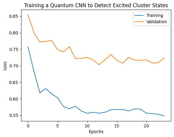
plt.plot(history.history['loss'][1:], label='Training')
plt.plot(history.history['val_loss'][1:], label='Validation')
plt.title('Training a Quantum CNN to Detect Excited Cluster States')
plt.xlabel('Epochs')
plt.ylabel('Loss')
plt.legend()
plt.show()
2. 混合模型
您不必使用量子卷積從八個量子位元減少到一個量子位元 - 您可以執行一或兩輪量子卷積,並將結果饋送到傳統神經網路。本節探討量子-傳統混合模型。
2.1 具有單一量子篩選器的混合模型
套用一層量子卷積,在所有位元上讀取 \(\langle \hat{Z}_n \rangle\),然後是密集連線的神經網路。
2.1.1 模型定義
# 1-local operators to read out
readouts = [cirq.Z(bit) for bit in cluster_state_bits[4:]]
def multi_readout_model_circuit(qubits):
"""Make a model circuit with less quantum pool and conv operations."""
model_circuit = cirq.Circuit()
symbols = sympy.symbols('qconv0:21')
model_circuit += quantum_conv_circuit(qubits, symbols[0:15])
model_circuit += quantum_pool_circuit(qubits[:4], qubits[4:],
symbols[15:21])
return model_circuit
# Build a model enacting the logic in 2.1 of this notebook.
excitation_input_dual = tf.keras.Input(shape=(), dtype=tf.dtypes.string)
cluster_state_dual = tfq.layers.AddCircuit()(
excitation_input_dual, prepend=cluster_state_circuit(cluster_state_bits))
quantum_model_dual = tfq.layers.PQC(
multi_readout_model_circuit(cluster_state_bits),
readouts)(cluster_state_dual)
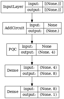
d1_dual = tf.keras.layers.Dense(8)(quantum_model_dual)
d2_dual = tf.keras.layers.Dense(1)(d1_dual)
hybrid_model = tf.keras.Model(inputs=[excitation_input_dual], outputs=[d2_dual])
# Display the model architecture
tf.keras.utils.plot_model(hybrid_model,
show_shapes=True,
show_layer_names=False,
dpi=70)
/tmpfs/src/tf_docs_env/lib/python3.9/site-packages/keras/src/initializers/initializers.py:120: UserWarning: The initializer RandomUniform is unseeded and being called multiple times, which will return identical values each time (even if the initializer is unseeded). Please update your code to provide a seed to the initializer, or avoid using the same initializer instance more than once.
  warnings.warn(
2.1.2 訓練模型
hybrid_model.compile(optimizer=tf.keras.optimizers.Adam(learning_rate=0.02),
                     loss=tf.losses.mse,
                     metrics=[custom_accuracy])

hybrid_history = hybrid_model.fit(x=train_excitations,
                                  y=train_labels,
                                  batch_size=16,
                                  epochs=25,
                                  verbose=1,
                                  validation_data=(test_excitations,
                                                   test_labels))
Epoch 1/25
7/7 [==============================] - 1s 100ms/step - loss: 0.6982 - custom_accuracy: 0.7589 - val_loss: 0.5877 - val_custom_accuracy: 0.7708
Epoch 2/25
7/7 [==============================] - 0s 68ms/step - loss: 0.2746 - custom_accuracy: 0.9554 - val_loss: 0.3261 - val_custom_accuracy: 0.9167
Epoch 3/25
7/7 [==============================] - 0s 66ms/step - loss: 0.2351 - custom_accuracy: 0.9464 - val_loss: 0.3478 - val_custom_accuracy: 0.9375
Epoch 4/25
7/7 [==============================] - 0s 67ms/step - loss: 0.2033 - custom_accuracy: 0.9554 - val_loss: 0.2885 - val_custom_accuracy: 0.9375
Epoch 5/25
7/7 [==============================] - 0s 65ms/step - loss: 0.2024 - custom_accuracy: 0.9554 - val_loss: 0.3089 - val_custom_accuracy: 0.9792
Epoch 6/25
7/7 [==============================] - 0s 64ms/step - loss: 0.1904 - custom_accuracy: 0.9911 - val_loss: 0.2340 - val_custom_accuracy: 1.0000
Epoch 7/25
7/7 [==============================] - 0s 64ms/step - loss: 0.1717 - custom_accuracy: 0.9732 - val_loss: 0.2339 - val_custom_accuracy: 1.0000
Epoch 8/25
7/7 [==============================] - 0s 64ms/step - loss: 0.1827 - custom_accuracy: 0.9821 - val_loss: 0.2440 - val_custom_accuracy: 1.0000
Epoch 9/25
7/7 [==============================] - 0s 64ms/step - loss: 0.1881 - custom_accuracy: 0.9821 - val_loss: 0.2371 - val_custom_accuracy: 1.0000
Epoch 10/25
7/7 [==============================] - 0s 64ms/step - loss: 0.1814 - custom_accuracy: 0.9911 - val_loss: 0.2549 - val_custom_accuracy: 1.0000
Epoch 11/25
7/7 [==============================] - 0s 64ms/step - loss: 0.1745 - custom_accuracy: 0.9911 - val_loss: 0.2521 - val_custom_accuracy: 0.9583
Epoch 12/25
7/7 [==============================] - 0s 64ms/step - loss: 0.1726 - custom_accuracy: 0.9911 - val_loss: 0.2241 - val_custom_accuracy: 1.0000
Epoch 13/25
7/7 [==============================] - 0s 65ms/step - loss: 0.1775 - custom_accuracy: 0.9911 - val_loss: 0.2386 - val_custom_accuracy: 0.9792
Epoch 14/25
7/7 [==============================] - 0s 63ms/step - loss: 0.2061 - custom_accuracy: 0.9643 - val_loss: 0.2496 - val_custom_accuracy: 1.0000
Epoch 15/25
7/7 [==============================] - 0s 63ms/step - loss: 0.1840 - custom_accuracy: 0.9821 - val_loss: 0.3156 - val_custom_accuracy: 0.9375
Epoch 16/25
7/7 [==============================] - 0s 63ms/step - loss: 0.1860 - custom_accuracy: 0.9821 - val_loss: 0.2323 - val_custom_accuracy: 0.9792
Epoch 17/25
7/7 [==============================] - 0s 63ms/step - loss: 0.1755 - custom_accuracy: 0.9911 - val_loss: 0.2253 - val_custom_accuracy: 1.0000
Epoch 18/25
7/7 [==============================] - 0s 63ms/step - loss: 0.1917 - custom_accuracy: 0.9732 - val_loss: 0.2386 - val_custom_accuracy: 1.0000
Epoch 19/25
7/7 [==============================] - 0s 62ms/step - loss: 0.1814 - custom_accuracy: 0.9911 - val_loss: 0.2515 - val_custom_accuracy: 0.9792
Epoch 20/25
7/7 [==============================] - 0s 63ms/step - loss: 0.1899 - custom_accuracy: 0.9643 - val_loss: 0.2307 - val_custom_accuracy: 0.9792
Epoch 21/25
7/7 [==============================] - 0s 63ms/step - loss: 0.1722 - custom_accuracy: 0.9911 - val_loss: 0.2353 - val_custom_accuracy: 1.0000
Epoch 22/25
7/7 [==============================] - 0s 64ms/step - loss: 0.1755 - custom_accuracy: 0.9732 - val_loss: 0.2237 - val_custom_accuracy: 1.0000
Epoch 23/25
7/7 [==============================] - 0s 63ms/step - loss: 0.1973 - custom_accuracy: 0.9821 - val_loss: 0.2977 - val_custom_accuracy: 0.9792
Epoch 24/25
7/7 [==============================] - 0s 63ms/step - loss: 0.1862 - custom_accuracy: 0.9821 - val_loss: 0.2310 - val_custom_accuracy: 0.9792
Epoch 25/25
7/7 [==============================] - 0s 63ms/step - loss: 0.1853 - custom_accuracy: 0.9821 - val_loss: 0.2680 - val_custom_accuracy: 0.9792
plt.plot(history.history['val_custom_accuracy'], label='QCNN')
plt.plot(hybrid_history.history['val_custom_accuracy'], label='Hybrid CNN')
plt.title('Quantum vs Hybrid CNN performance')
plt.xlabel('Epochs')
plt.legend()
plt.ylabel('Validation Accuracy')
plt.show()
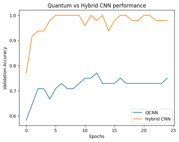
您可以看到,在非常適度的傳統輔助下,混合模型通常比純粹的量子版本收斂得更快。
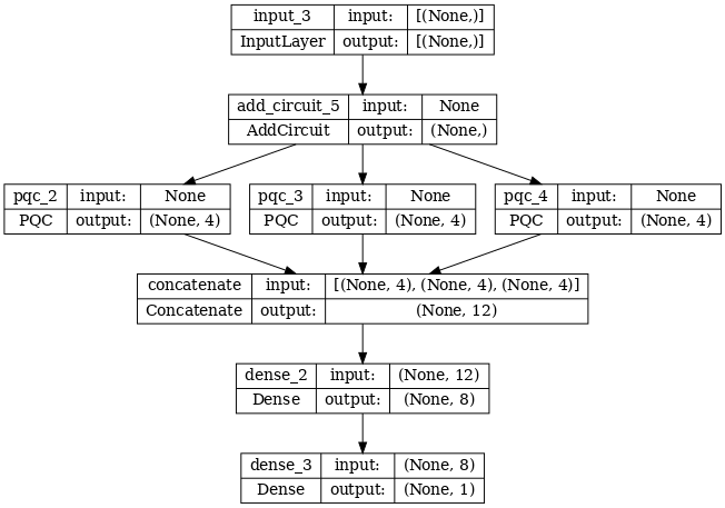
2.2 具有多個量子篩選器的混合卷積
現在讓我們嘗試一種架構,該架構使用多個量子卷積和傳統神經網路來組合它們。
2.2.1 模型定義
excitation_input_multi = tf.keras.Input(shape=(), dtype=tf.dtypes.string)

cluster_state_multi = tfq.layers.AddCircuit()(
    excitation_input_multi, prepend=cluster_state_circuit(cluster_state_bits))

# apply 3 different filters and measure expectation values

quantum_model_multi1 = tfq.layers.PQC(
    multi_readout_model_circuit(cluster_state_bits),
    readouts)(cluster_state_multi)

quantum_model_multi2 = tfq.layers.PQC(
    multi_readout_model_circuit(cluster_state_bits),
    readouts)(cluster_state_multi)

quantum_model_multi3 = tfq.layers.PQC(
    multi_readout_model_circuit(cluster_state_bits),
    readouts)(cluster_state_multi)

# concatenate outputs and feed into a small classical NN
concat_out = tf.keras.layers.concatenate(
    [quantum_model_multi1, quantum_model_multi2, quantum_model_multi3])

dense_1 = tf.keras.layers.Dense(8)(concat_out)

dense_2 = tf.keras.layers.Dense(1)(dense_1)

multi_qconv_model = tf.keras.Model(inputs=[excitation_input_multi],
                                   outputs=[dense_2])

# Display the model architecture
tf.keras.utils.plot_model(multi_qconv_model,
                          show_shapes=True,
                          show_layer_names=True,
                          dpi=70)
/tmpfs/src/tf_docs_env/lib/python3.9/site-packages/keras/src/initializers/initializers.py:120: UserWarning: The initializer RandomUniform is unseeded and being called multiple times, which will return identical values each time (even if the initializer is unseeded). Please update your code to provide a seed to the initializer, or avoid using the same initializer instance more than once.
  warnings.warn(
2.2.2 訓練模型
multi_qconv_model.compile(
    optimizer=tf.keras.optimizers.Adam(learning_rate=0.02),
    loss=tf.losses.mse,
    metrics=[custom_accuracy])

multi_qconv_history = multi_qconv_model.fit(x=train_excitations,
                                            y=train_labels,
                                            batch_size=16,
                                            epochs=25,
                                            verbose=1,
                                            validation_data=(test_excitations,
                                                             test_labels))
Epoch 1/25
7/7 [==============================] - 2s 116ms/step - loss: 0.6554 - custom_accuracy: 0.7857 - val_loss: 0.4377 - val_custom_accuracy: 0.8958
Epoch 2/25
7/7 [==============================] - 0s 74ms/step - loss: 0.2390 - custom_accuracy: 0.9375 - val_loss: 0.2941 - val_custom_accuracy: 0.9375
Epoch 3/25
7/7 [==============================] - 1s 79ms/step - loss: 0.2300 - custom_accuracy: 0.9643 - val_loss: 0.2889 - val_custom_accuracy: 0.9583
Epoch 4/25
7/7 [==============================] - 0s 72ms/step - loss: 0.1848 - custom_accuracy: 0.9821 - val_loss: 0.2479 - val_custom_accuracy: 0.9792
Epoch 5/25
7/7 [==============================] - 0s 72ms/step - loss: 0.1928 - custom_accuracy: 0.9821 - val_loss: 0.2408 - val_custom_accuracy: 0.9792
Epoch 6/25
7/7 [==============================] - 1s 77ms/step - loss: 0.1789 - custom_accuracy: 0.9821 - val_loss: 0.2372 - val_custom_accuracy: 1.0000
Epoch 7/25
7/7 [==============================] - 0s 69ms/step - loss: 0.1675 - custom_accuracy: 0.9821 - val_loss: 0.2517 - val_custom_accuracy: 1.0000
Epoch 8/25
7/7 [==============================] - 0s 71ms/step - loss: 0.1608 - custom_accuracy: 0.9911 - val_loss: 0.2438 - val_custom_accuracy: 1.0000
Epoch 9/25
7/7 [==============================] - 0s 70ms/step - loss: 0.1718 - custom_accuracy: 0.9821 - val_loss: 0.2568 - val_custom_accuracy: 0.9792
Epoch 10/25
7/7 [==============================] - 0s 73ms/step - loss: 0.1780 - custom_accuracy: 0.9821 - val_loss: 0.2741 - val_custom_accuracy: 0.9792
Epoch 11/25
7/7 [==============================] - 0s 70ms/step - loss: 0.1794 - custom_accuracy: 0.9911 - val_loss: 0.2458 - val_custom_accuracy: 0.9792
Epoch 12/25
7/7 [==============================] - 0s 70ms/step - loss: 0.1843 - custom_accuracy: 0.9821 - val_loss: 0.2515 - val_custom_accuracy: 0.9792
Epoch 13/25
7/7 [==============================] - 1s 71ms/step - loss: 0.1775 - custom_accuracy: 0.9911 - val_loss: 0.2820 - val_custom_accuracy: 0.9792
Epoch 14/25
7/7 [==============================] - 0s 72ms/step - loss: 0.1771 - custom_accuracy: 0.9911 - val_loss: 0.2586 - val_custom_accuracy: 1.0000
Epoch 15/25
7/7 [==============================] - 1s 79ms/step - loss: 0.1665 - custom_accuracy: 0.9732 - val_loss: 0.2348 - val_custom_accuracy: 1.0000
Epoch 16/25
7/7 [==============================] - 0s 73ms/step - loss: 0.1962 - custom_accuracy: 0.9732 - val_loss: 0.2533 - val_custom_accuracy: 0.9792
Epoch 17/25
7/7 [==============================] - 1s 79ms/step - loss: 0.1769 - custom_accuracy: 0.9911 - val_loss: 0.2565 - val_custom_accuracy: 0.9792
Epoch 18/25
7/7 [==============================] - 1s 74ms/step - loss: 0.1648 - custom_accuracy: 0.9911 - val_loss: 0.2618 - val_custom_accuracy: 0.9583
Epoch 19/25
7/7 [==============================] - 0s 71ms/step - loss: 0.1722 - custom_accuracy: 0.9732 - val_loss: 0.2442 - val_custom_accuracy: 0.9792
Epoch 20/25
7/7 [==============================] - 1s 78ms/step - loss: 0.1646 - custom_accuracy: 0.9732 - val_loss: 0.2327 - val_custom_accuracy: 0.9792
Epoch 21/25
7/7 [==============================] - 0s 70ms/step - loss: 0.1632 - custom_accuracy: 0.9732 - val_loss: 0.2418 - val_custom_accuracy: 0.9792
Epoch 22/25
7/7 [==============================] - 0s 71ms/step - loss: 0.1560 - custom_accuracy: 0.9911 - val_loss: 0.2440 - val_custom_accuracy: 1.0000
Epoch 23/25
7/7 [==============================] - 0s 72ms/step - loss: 0.1594 - custom_accuracy: 0.9821 - val_loss: 0.2495 - val_custom_accuracy: 0.9375
Epoch 24/25
7/7 [==============================] - 1s 80ms/step - loss: 0.1669 - custom_accuracy: 0.9821 - val_loss: 0.3298 - val_custom_accuracy: 0.9583
Epoch 25/25
7/7 [==============================] - 0s 68ms/step - loss: 0.1758 - custom_accuracy: 0.9821 - val_loss: 0.2492 - val_custom_accuracy: 0.9792
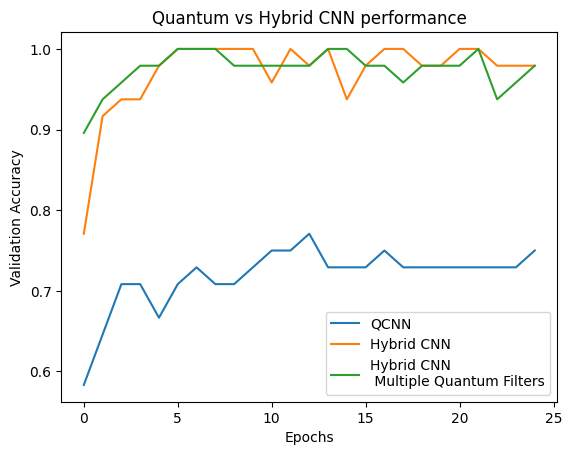
plt.plot(history.history['val_custom_accuracy'][:25], label='QCNN')
plt.plot(hybrid_history.history['val_custom_accuracy'][:25], label='Hybrid CNN')
plt.plot(multi_qconv_history.history['val_custom_accuracy'][:25],
         label='Hybrid CNN \n Multiple Quantum Filters')
plt.title('Quantum vs Hybrid CNN performance')
plt.xlabel('Epochs')
plt.legend()
plt.ylabel('Validation Accuracy')
plt.show()