|
|
|
 在 GitHub 上檢視原始碼 在 GitHub 上檢視原始碼
|
|
本教學課程建構量子神經網路 (QNN),以分類簡化版的 MNIST,類似於 Farhi 等人 使用的方法。量子神經網路在這個傳統資料問題上的效能會與傳統神經網路比較。
設定
pip install tensorflow==2.15.0
安裝 TensorFlow Quantum
pip install tensorflow-quantum==0.7.3
# Update package resources to account for version changes.
import importlib, pkg_resources
importlib.reload(pkg_resources)
/tmpfs/tmp/ipykernel_23360/1875984233.py:2: DeprecationWarning: pkg_resources is deprecated as an API. See https://setuptools.pypa.io/en/latest/pkg_resources.html
  import importlib, pkg_resources
<module 'pkg_resources' from '/tmpfs/src/tf_docs_env/lib/python3.9/site-packages/pkg_resources/__init__.py'>
現在匯入 TensorFlow 和模組依附元件
import tensorflow as tf
import tensorflow_quantum as tfq

import cirq
import sympy
import numpy as np
import seaborn as sns
import collections

# visualization tools
%matplotlib inline
import matplotlib.pyplot as plt
from cirq.contrib.svg import SVGCircuit
2024-05-18 11:39:20.065737: E external/local_xla/xla/stream_executor/cuda/cuda_dnn.cc:9261] Unable to register cuDNN factory: Attempting to register factory for plugin cuDNN when one has already been registered
2024-05-18 11:39:20.065786: E external/local_xla/xla/stream_executor/cuda/cuda_fft.cc:607] Unable to register cuFFT factory: Attempting to register factory for plugin cuFFT when one has already been registered
2024-05-18 11:39:20.067281: E external/local_xla/xla/stream_executor/cuda/cuda_blas.cc:1515] Unable to register cuBLAS factory: Attempting to register factory for plugin cuBLAS when one has already been registered
2024-05-18 11:39:23.413260: E external/local_xla/xla/stream_executor/cuda/cuda_driver.cc:274] failed call to cuInit: CUDA_ERROR_NO_DEVICE: no CUDA-capable device is detected
1. 載入資料
在本教學課程中,您將建構二元分類器,以區分數字 3 和 6,遵循 Farhi 等人 的做法。本節涵蓋資料處理,其
- 從 Keras 載入原始資料。
- 篩選資料集,僅保留 3 和 6。
- 縮小圖片尺寸,使其能符合量子電腦。
- 移除任何矛盾的範例。
- 將二元圖片轉換為 Cirq 電路。
- 將 Cirq 電路轉換為 TensorFlow Quantum 電路。
1.1 載入原始資料
載入與 Keras 一起散佈的 MNIST 資料集。
(x_train, y_train), (x_test, y_test) = tf.keras.datasets.mnist.load_data()

# Rescale the images from [0,255] to the [0.0,1.0] range.
x_train, x_test = x_train[..., np.newaxis]/255.0, x_test[..., np.newaxis]/255.0

print("Number of original training examples:", len(x_train))
print("Number of original test examples:", len(x_test))
Downloading data from https://storage.googleapis.com/tensorflow/tf-keras-datasets/mnist.npz
11490434/11490434 [==============================] - 0s 0us/step
Number of original training examples: 60000
Number of original test examples: 10000
篩選資料集,僅保留 3 和 6,移除其他類別。同時轉換標籤 y 為布林值:True 代表 3,False 代表 6。
def filter_36(x, y):
    keep = (y == 3) | (y == 6)
    x, y = x[keep], y[keep]
    y = y == 3
    return x,y
x_train, y_train = filter_36(x_train, y_train)
x_test, y_test = filter_36(x_test, y_test)

print("Number of filtered training examples:", len(x_train))
print("Number of filtered test examples:", len(x_test))
Number of filtered training examples: 12049
Number of filtered test examples: 1968
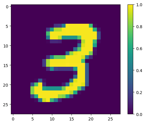
顯示第一個範例
print(y_train[0])

plt.imshow(x_train[0, :, :, 0])
plt.colorbar()
True
<matplotlib.colorbar.Colorbar at 0x7f68721d07f0>
1.2 縮小圖片尺寸
28x28 的圖片尺寸對於目前的量子電腦而言太大了。將圖片尺寸縮小為 4x4
x_train_small = tf.image.resize(x_train, (4,4)).numpy()
x_test_small = tf.image.resize(x_test, (4,4)).numpy()
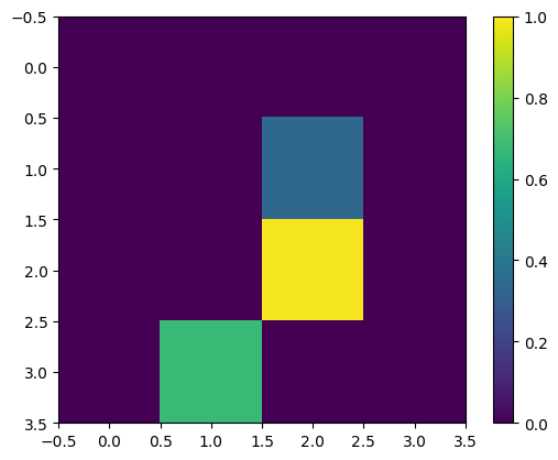
再次顯示第一個訓練範例 (調整尺寸後)
print(y_train[0])

plt.imshow(x_train_small[0,:,:,0], vmin=0, vmax=1)
plt.colorbar()
True
<matplotlib.colorbar.Colorbar at 0x7f6872141ca0>
1.3 移除矛盾的範例
從 Farhi 等人 的第 3.3 節:學習區分數字 中,篩選資料集以移除標記為同時屬於兩個類別的圖片。
這不是標準的機器學習程序,但為了遵循論文而納入。
def remove_contradicting(xs, ys):
    mapping = collections.defaultdict(set)
    orig_x = {}
    # Determine the set of labels for each unique image:
    for x,y in zip(xs,ys):
       orig_x[tuple(x.flatten())] = x
       mapping[tuple(x.flatten())].add(y)

    new_x = []
    new_y = []
    for flatten_x in mapping:
      x = orig_x[flatten_x]
      labels = mapping[flatten_x]
      if len(labels) == 1:
          new_x.append(x)
          new_y.append(next(iter(labels)))
      else:
          # Throw out images that match more than one label.
          pass

    num_uniq_3 = sum(1 for value in mapping.values() if len(value) == 1 and True in value)
    num_uniq_6 = sum(1 for value in mapping.values() if len(value) == 1 and False in value)
    num_uniq_both = sum(1 for value in mapping.values() if len(value) == 2)

    print("Number of unique images:", len(mapping.values()))
    print("Number of unique 3s: ", num_uniq_3)
    print("Number of unique 6s: ", num_uniq_6)
    print("Number of unique contradicting labels (both 3 and 6): ", num_uniq_both)
    print()
    print("Initial number of images: ", len(xs))
    print("Remaining non-contradicting unique images: ", len(new_x))

    return np.array(new_x), np.array(new_y)
產生的計數與報告的值並不完全相符,但未指定確切的程序。
同樣值得注意的是,在此時套用篩選矛盾範例並不能完全防止模型接收矛盾的訓練範例:下一步驟會將資料二元化,這會導致更多衝突。
x_train_nocon, y_train_nocon = remove_contradicting(x_train_small, y_train)
Number of unique images: 10387
Number of unique 3s:  4912
Number of unique 6s:  5426
Number of unique contradicting labels (both 3 and 6):  49

Initial number of images:  12049
Remaining non-contradicting unique images:  10338
1.4 將資料編碼為量子電路
為了使用量子電腦處理圖片,Farhi 等人 提出以量子位元表示每個像素,其狀態取決於像素的值。第一步是轉換為二元編碼。
THRESHOLD = 0.5

x_train_bin = np.array(x_train_nocon > THRESHOLD, dtype=np.float32)
x_test_bin = np.array(x_test_small > THRESHOLD, dtype=np.float32)
如果您在此時移除矛盾的圖片,則只會剩下 193 張,可能不足以進行有效的訓練。
_ = remove_contradicting(x_train_bin, y_train_nocon)
Number of unique images: 193
Number of unique 3s:  80
Number of unique 6s:  69
Number of unique contradicting labels (both 3 and 6):  44

Initial number of images:  10338
Remaining non-contradicting unique images:  149
像素索引處的值超過閾值的量子位元會透過 \(X\) 閘旋轉。
def convert_to_circuit(image):
    """Encode truncated classical image into quantum datapoint."""
    values = np.ndarray.flatten(image)
    qubits = cirq.GridQubit.rect(4, 4)
    circuit = cirq.Circuit()
    for i, value in enumerate(values):
        if value:
            circuit.append(cirq.X(qubits[i]))
    return circuit


x_train_circ = [convert_to_circuit(x) for x in x_train_bin]
x_test_circ = [convert_to_circuit(x) for x in x_test_bin]
以下是為第一個範例建立的電路 (電路圖未顯示零閘的量子位元)
SVGCircuit(x_train_circ[0])
findfont: Font family 'Arial' not found.
findfont: Font family 'Arial' not found.
findfont: Font family 'Arial' not found.
findfont: Font family 'Arial' not found.

將此電路與圖片值超過閾值的索引進行比較
bin_img = x_train_bin[0,:,:,0]
indices = np.array(np.where(bin_img)).T
indices
array([[2, 2],
       [3, 1]])
將這些 Cirq 電路轉換為 tfq 的張量
x_train_tfcirc = tfq.convert_to_tensor(x_train_circ)
x_test_tfcirc = tfq.convert_to_tensor(x_test_circ)
2. 量子神經網路
對於分類圖片的量子電路結構,幾乎沒有任何指導。由於分類是以讀出量子位元的期望值為基礎,Farhi 等人 建議使用雙量子位元閘,且讀出量子位元始終受作用。這在某些方面類似於跨像素執行小型 Unitary RNN。
2.1 建構模型電路
以下範例顯示此分層方法。每一層都使用相同閘的 n 個執行個體,其中每個資料量子位元都作用於讀出量子位元。
從一個簡單的類別開始,它會將這些閘層新增至電路
class CircuitLayerBuilder():
    def __init__(self, data_qubits, readout):
        self.data_qubits = data_qubits
        self.readout = readout

    def add_layer(self, circuit, gate, prefix):
        for i, qubit in enumerate(self.data_qubits):
            symbol = sympy.Symbol(prefix + '-' + str(i))
            circuit.append(gate(qubit, self.readout)**symbol)
建構範例電路層以查看其外觀
demo_builder = CircuitLayerBuilder(data_qubits = cirq.GridQubit.rect(4,1),
                                   readout=cirq.GridQubit(-1,-1))

circuit = cirq.Circuit()
demo_builder.add_layer(circuit, gate = cirq.XX, prefix='xx')
SVGCircuit(circuit)
findfont: Font family 'Arial' not found.
findfont: Font family 'Arial' not found.
findfont: Font family 'Arial' not found.
findfont: Font family 'Arial' not found.
findfont: Font family 'Arial' not found.
findfont: Font family 'Arial' not found.
findfont: Font family 'Arial' not found.
findfont: Font family 'Arial' not found.
findfont: Font family 'Arial' not found.
findfont: Font family 'Arial' not found.
findfont: Font family 'Arial' not found.
findfont: Font family 'Arial' not found.
findfont: Font family 'Arial' not found.

現在建構一個雙層模型,使其與資料電路尺寸相符,並納入準備和讀出運算。
def create_quantum_model():
    """Create a QNN model circuit and readout operation to go along with it."""
    data_qubits = cirq.GridQubit.rect(4, 4)  # a 4x4 grid.
    readout = cirq.GridQubit(-1, -1)         # a single qubit at [-1,-1]
    circuit = cirq.Circuit()

    # Prepare the readout qubit.
    circuit.append(cirq.X(readout))
    circuit.append(cirq.H(readout))

    builder = CircuitLayerBuilder(
        data_qubits = data_qubits,
        readout=readout)

    # Then add layers (experiment by adding more).
    builder.add_layer(circuit, cirq.XX, "xx1")
    builder.add_layer(circuit, cirq.ZZ, "zz1")

    # Finally, prepare the readout qubit.
    circuit.append(cirq.H(readout))

    return circuit, cirq.Z(readout)
model_circuit, model_readout = create_quantum_model()
2.2 將模型電路包裝在 tfq-keras 模型中
使用量子元件建構 Keras 模型。此模型會饋送來自 x_train_circ 的「量子資料」,其編碼傳統資料。它使用參數化量子電路層 tfq.layers.PQC,以在量子資料上訓練模型電路。
為了分類這些圖片,Farhi 等人 建議取得參數化電路中讀出量子位元的期望值。期望值會傳回介於 1 和 -1 之間的值。
# Build the Keras model.
model = tf.keras.Sequential([
    # The input is the data-circuit, encoded as a tf.string
    tf.keras.layers.Input(shape=(), dtype=tf.string),
    # The PQC layer returns the expected value of the readout gate, range [-1,1].
    tfq.layers.PQC(model_circuit, model_readout),
])
接下來,使用 compile 方法描述模型的訓練程序。
由於預期的讀出值在 [-1,1] 範圍內,因此最佳化 hinge 損失在某種程度上是自然而然的選擇。
若要在此處使用 hinge 損失,您需要進行兩項小調整。首先,將標籤 y_train_nocon 從布林值轉換為 [-1,1],這是 hinge 損失預期的值。
y_train_hinge = 2.0*y_train_nocon-1.0
y_test_hinge = 2.0*y_test-1.0
其次,使用自訂 hinge_accuracy 指標,正確處理 [-1, 1] 作為 y_true 標籤引數。tf.losses.BinaryAccuracy(threshold=0.0) 預期 y_true 為布林值,因此不能與 hinge 損失搭配使用)。
def hinge_accuracy(y_true, y_pred):
    y_true = tf.squeeze(y_true) > 0.0
    y_pred = tf.squeeze(y_pred) > 0.0
    result = tf.cast(y_true == y_pred, tf.float32)

    return tf.reduce_mean(result)
model.compile(
    loss=tf.keras.losses.Hinge(),
    optimizer=tf.keras.optimizers.Adam(),
    metrics=[hinge_accuracy])
print(model.summary())
Model: "sequential"
_________________________________________________________________
 Layer (type)                Output Shape              Param #
=================================================================
 pqc (PQC)                   (None, 1)                 32

=================================================================
Total params: 32 (128.00 Byte)
Trainable params: 32 (128.00 Byte)
Non-trainable params: 0 (0.00 Byte)
_________________________________________________________________
None
訓練量子模型
現在訓練模型,這大約需要 45 分鐘。如果您不想等待那麼久,請使用資料的小子集 (在下方設定 NUM_EXAMPLES=500)。這實際上不會影響模型在訓練期間的進度 (它只有 32 個參數,不需要太多資料來限制這些參數)。使用較少的範例只會提早結束訓練 (5 分鐘),但執行時間夠長,足以顯示它在驗證記錄中取得進展。
EPOCHS = 3
BATCH_SIZE = 32

NUM_EXAMPLES = len(x_train_tfcirc)
x_train_tfcirc_sub = x_train_tfcirc[:NUM_EXAMPLES]
y_train_hinge_sub = y_train_hinge[:NUM_EXAMPLES]
將此模型訓練至收斂應該可以在測試集上達到 >85% 的準確度。
qnn_history = model.fit(
      x_train_tfcirc_sub, y_train_hinge_sub,
      batch_size=32,
      epochs=EPOCHS,
      verbose=1,
      validation_data=(x_test_tfcirc, y_test_hinge))

qnn_results = model.evaluate(x_test_tfcirc, y_test)
Epoch 1/3
324/324 [==============================] - 56s 172ms/step - loss: 0.7905 - hinge_accuracy: 0.6830 - val_loss: 0.4799 - val_hinge_accuracy: 0.7666
Epoch 2/3
324/324 [==============================] - 55s 171ms/step - loss: 0.4111 - hinge_accuracy: 0.8091 - val_loss: 0.3706 - val_hinge_accuracy: 0.8266
Epoch 3/3
324/324 [==============================] - 55s 171ms/step - loss: 0.3588 - hinge_accuracy: 0.8801 - val_loss: 0.3472 - val_hinge_accuracy: 0.9042
62/62 [==============================] - 2s 32ms/step - loss: 0.3472 - hinge_accuracy: 0.9042
3. 傳統神經網路
雖然量子神經網路適用於這個簡化的 MNIST 問題,但基本傳統神經網路可以輕鬆地在這個任務上勝過 QNN。在單一 epoch 之後,傳統神經網路可以在保留集上達到 >98% 的準確度。
在以下範例中,傳統神經網路用於 3-6 分類問題,使用完整的 28x28 圖片,而不是對圖片進行子取樣。這很容易收斂到接近 100% 的測試集準確度。
def create_classical_model():
    # A simple model based off LeNet from https://keras.dev.org.tw/examples/mnist_cnn/
    model = tf.keras.Sequential()
    model.add(tf.keras.layers.Conv2D(32, [3, 3], activation='relu', input_shape=(28,28,1)))
    model.add(tf.keras.layers.Conv2D(64, [3, 3], activation='relu'))
    model.add(tf.keras.layers.MaxPooling2D(pool_size=(2, 2)))
    model.add(tf.keras.layers.Dropout(0.25))
    model.add(tf.keras.layers.Flatten())
    model.add(tf.keras.layers.Dense(128, activation='relu'))
    model.add(tf.keras.layers.Dropout(0.5))
    model.add(tf.keras.layers.Dense(1))
    return model


model = create_classical_model()
model.compile(loss=tf.keras.losses.BinaryCrossentropy(from_logits=True),
              optimizer=tf.keras.optimizers.Adam(),
              metrics=['accuracy'])

model.summary()
Model: "sequential_1"
_________________________________________________________________
 Layer (type)                Output Shape              Param #
=================================================================
 conv2d (Conv2D)             (None, 26, 26, 32)        320

 conv2d_1 (Conv2D)           (None, 24, 24, 64)        18496

 max_pooling2d (MaxPooling2  (None, 12, 12, 64)        0
 D)

 dropout (Dropout)           (None, 12, 12, 64)        0

 flatten (Flatten)           (None, 9216)              0

 dense (Dense)               (None, 128)               1179776

 dropout_1 (Dropout)         (None, 128)               0

 dense_1 (Dense)             (None, 1)                 129

=================================================================
Total params: 1198721 (4.57 MB)
Trainable params: 1198721 (4.57 MB)
Non-trainable params: 0 (0.00 Byte)
_________________________________________________________________
model.fit(x_train,
          y_train,
          batch_size=128,
          epochs=1,
          verbose=1,
          validation_data=(x_test, y_test))

cnn_results = model.evaluate(x_test, y_test)
95/95 [==============================] - 3s 27ms/step - loss: 0.0440 - accuracy: 0.9839 - val_loss: 0.0025 - val_accuracy: 0.9995
62/62 [==============================] - 0s 3ms/step - loss: 0.0025 - accuracy: 0.9995
上述模型有將近 120 萬個參數。為了更公平的比較,請嘗試在子取樣圖片上使用 37 個參數的模型
def create_fair_classical_model():
    # A simple model based off LeNet from https://keras.dev.org.tw/examples/mnist_cnn/
    model = tf.keras.Sequential()
    model.add(tf.keras.layers.Flatten(input_shape=(4,4,1)))
    model.add(tf.keras.layers.Dense(2, activation='relu'))
    model.add(tf.keras.layers.Dense(1))
    return model


model = create_fair_classical_model()
model.compile(loss=tf.keras.losses.BinaryCrossentropy(from_logits=True),
              optimizer=tf.keras.optimizers.Adam(),
              metrics=['accuracy'])

model.summary()
Model: "sequential_2"
_________________________________________________________________
 Layer (type)                Output Shape              Param #
=================================================================
 flatten_1 (Flatten)         (None, 16)                0

 dense_2 (Dense)             (None, 2)                 34

 dense_3 (Dense)             (None, 1)                 3

=================================================================
Total params: 37 (148.00 Byte)
Trainable params: 37 (148.00 Byte)
Non-trainable params: 0 (0.00 Byte)
_________________________________________________________________
model.fit(x_train_bin,
          y_train_nocon,
          batch_size=128,
          epochs=20,
          verbose=2,
          validation_data=(x_test_bin, y_test))

fair_nn_results = model.evaluate(x_test_bin, y_test)
Epoch 1/20
81/81 - 1s - loss: 0.7028 - accuracy: 0.4897 - val_loss: 0.6585 - val_accuracy: 0.4949 - 782ms/epoch - 10ms/step
Epoch 2/20
81/81 - 0s - loss: 0.6561 - accuracy: 0.5311 - val_loss: 0.6067 - val_accuracy: 0.4990 - 124ms/epoch - 2ms/step
Epoch 3/20
81/81 - 0s - loss: 0.5895 - accuracy: 0.5903 - val_loss: 0.5275 - val_accuracy: 0.6489 - 119ms/epoch - 1ms/step
Epoch 4/20
81/81 - 0s - loss: 0.5095 - accuracy: 0.7001 - val_loss: 0.4511 - val_accuracy: 0.7571 - 121ms/epoch - 1ms/step
Epoch 5/20
81/81 - 0s - loss: 0.4385 - accuracy: 0.7760 - val_loss: 0.3908 - val_accuracy: 0.7749 - 122ms/epoch - 2ms/step
Epoch 6/20
81/81 - 0s - loss: 0.3836 - accuracy: 0.8060 - val_loss: 0.3461 - val_accuracy: 0.8272 - 120ms/epoch - 1ms/step
Epoch 7/20
81/81 - 0s - loss: 0.3428 - accuracy: 0.8214 - val_loss: 0.3130 - val_accuracy: 0.8430 - 119ms/epoch - 1ms/step
Epoch 8/20
81/81 - 0s - loss: 0.3128 - accuracy: 0.8590 - val_loss: 0.2893 - val_accuracy: 0.8674 - 119ms/epoch - 1ms/step
Epoch 9/20
81/81 - 0s - loss: 0.2907 - accuracy: 0.8692 - val_loss: 0.2719 - val_accuracy: 0.8684 - 117ms/epoch - 1ms/step
Epoch 10/20
81/81 - 0s - loss: 0.2745 - accuracy: 0.8716 - val_loss: 0.2590 - val_accuracy: 0.8679 - 117ms/epoch - 1ms/step
Epoch 11/20
81/81 - 0s - loss: 0.2624 - accuracy: 0.8721 - val_loss: 0.2494 - val_accuracy: 0.8679 - 122ms/epoch - 2ms/step
Epoch 12/20
81/81 - 0s - loss: 0.2533 - accuracy: 0.8734 - val_loss: 0.2421 - val_accuracy: 0.8694 - 122ms/epoch - 2ms/step
Epoch 13/20
81/81 - 0s - loss: 0.2462 - accuracy: 0.8753 - val_loss: 0.2367 - val_accuracy: 0.8694 - 122ms/epoch - 2ms/step
Epoch 14/20
81/81 - 0s - loss: 0.2408 - accuracy: 0.8782 - val_loss: 0.2323 - val_accuracy: 0.8709 - 120ms/epoch - 1ms/step
Epoch 15/20
81/81 - 0s - loss: 0.2366 - accuracy: 0.8793 - val_loss: 0.2292 - val_accuracy: 0.8709 - 116ms/epoch - 1ms/step
Epoch 16/20
81/81 - 0s - loss: 0.2334 - accuracy: 0.8794 - val_loss: 0.2270 - val_accuracy: 0.8709 - 117ms/epoch - 1ms/step
Epoch 17/20
81/81 - 0s - loss: 0.2309 - accuracy: 0.8790 - val_loss: 0.2249 - val_accuracy: 0.8709 - 117ms/epoch - 1ms/step
Epoch 18/20
81/81 - 0s - loss: 0.2288 - accuracy: 0.8853 - val_loss: 0.2233 - val_accuracy: 0.9177 - 121ms/epoch - 1ms/step
Epoch 19/20
81/81 - 0s - loss: 0.2271 - accuracy: 0.8934 - val_loss: 0.2225 - val_accuracy: 0.8664 - 121ms/epoch - 1ms/step
Epoch 20/20
81/81 - 0s - loss: 0.2257 - accuracy: 0.8996 - val_loss: 0.2213 - val_accuracy: 0.9141 - 122ms/epoch - 2ms/step
62/62 [==============================] - 0s 1ms/step - loss: 0.2213 - accuracy: 0.9141
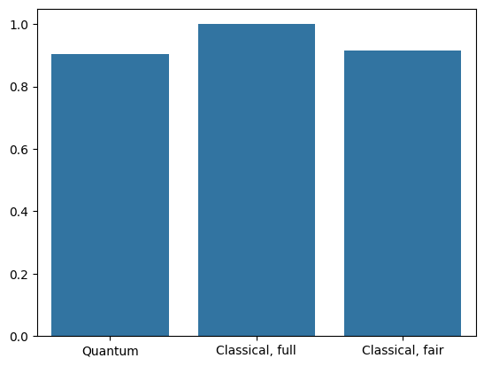
4. 比較
更高的解析度輸入和更強大的模型使 CNN 能夠輕鬆解決這個問題。雖然具有相似功率 (~32 個參數) 的傳統模型在極短的時間內訓練到相似的準確度。無論如何,傳統神經網路都輕鬆勝過量子神經網路。對於傳統資料而言,很難擊敗傳統神經網路。
qnn_accuracy = qnn_results[1]
cnn_accuracy = cnn_results[1]
fair_nn_accuracy = fair_nn_results[1]

sns.barplot(x=["Quantum", "Classical, full", "Classical, fair"],
            y=[qnn_accuracy, cnn_accuracy, fair_nn_accuracy])
<Axes: >