
|
|
|
 在 GitHub 上檢視原始碼 在 GitHub 上檢視原始碼
|
|
本教學課程說明古典神經網路如何學習修正量子位元校正錯誤。其中介紹了 Cirq,這是一個 Python 架構,可用於建立、編輯和叫用 Noisy Intermediate Scale Quantum (NISQ) 電路,並示範 Cirq 如何與 TensorFlow Quantum 介接。
設定
pip install tensorflow==2.15.0
安裝 TensorFlow Quantum
pip install tensorflow-quantum==0.7.3
# Update package resources to account for version changes.
import importlib, pkg_resources
importlib.reload(pkg_resources)
/tmpfs/tmp/ipykernel_11114/1875984233.py:2: DeprecationWarning: pkg_resources is deprecated as an API. See https://setuptools.pypa.io/en/latest/pkg_resources.html
  import importlib, pkg_resources
<module 'pkg_resources' from '/tmpfs/src/tf_docs_env/lib/python3.9/site-packages/pkg_resources/__init__.py'>
現在匯入 TensorFlow 和模組依附元件
import tensorflow as tf
import tensorflow_quantum as tfq

import cirq
import sympy
import numpy as np

# visualization tools
%matplotlib inline
import matplotlib.pyplot as plt
from cirq.contrib.svg import SVGCircuit
2024-05-18 11:22:39.011840: E external/local_xla/xla/stream_executor/cuda/cuda_dnn.cc:9261] Unable to register cuDNN factory: Attempting to register factory for plugin cuDNN when one has already been registered
2024-05-18 11:22:39.011885: E external/local_xla/xla/stream_executor/cuda/cuda_fft.cc:607] Unable to register cuFFT factory: Attempting to register factory for plugin cuFFT when one has already been registered
2024-05-18 11:22:39.013339: E external/local_xla/xla/stream_executor/cuda/cuda_blas.cc:1515] Unable to register cuBLAS factory: Attempting to register factory for plugin cuBLAS when one has already been registered
2024-05-18 11:22:42.671821: E external/local_xla/xla/stream_executor/cuda/cuda_driver.cc:274] failed call to cuInit: CUDA_ERROR_NO_DEVICE: no CUDA-capable device is detected
1. 基礎知識
1.1 Cirq 和參數化量子電路
在探索 TensorFlow Quantum (TFQ) 之前,我們先來看看一些 Cirq 基礎知識。Cirq 是 Google 推出的量子運算 Python 程式庫。您可以使用它來定義電路,包括靜態和參數化閘。
Cirq 使用 SymPy 符號來表示自由參數。
a, b = sympy.symbols('a b')
以下程式碼使用您的參數建立雙量子位元電路
# Create two qubits
q0, q1 = cirq.GridQubit.rect(1, 2)

# Create a circuit on these qubits using the parameters you created above.
circuit = cirq.Circuit(
    cirq.rx(a).on(q0),
    cirq.ry(b).on(q1), cirq.CNOT(q0, q1))

SVGCircuit(circuit)
findfont: Font family 'Arial' not found.
findfont: Font family 'Arial' not found.
findfont: Font family 'Arial' not found.
findfont: Font family 'Arial' not found.
findfont: Font family 'Arial' not found.
findfont: Font family 'Arial' not found.

若要評估電路,您可以使用 cirq.Simulator 介面。您可以傳入 cirq.ParamResolver 物件,以特定數字取代電路中的自由參數。以下程式碼會計算參數化電路的原始狀態向量輸出
# Calculate a state vector with a=0.5 and b=-0.5.
resolver = cirq.ParamResolver({a: 0.5, b: -0.5})
output_state_vector = cirq.Simulator().simulate(circuit, resolver).final_state_vector
output_state_vector
array([ 0.9387913 +0.j        , -0.23971277+0.j        ,

        0.        +0.06120872j,  0.        -0.23971277j], dtype=complex64)
狀態向量無法直接在模擬之外存取 (請注意上方輸出中的複數)。為了在物理上符合實際情況,您必須指定量測,將狀態向量轉換成古典電腦可以理解的實數。Cirq 使用 包立運算符 \(\hat{X}\)、\(\hat{Y}\) 和 \(\hat{Z}\) 的組合來指定量測。例如,以下程式碼會量測您剛模擬的狀態向量上的 \(\hat{Z}_0\) 和 \(\frac{1}{2}\hat{Z}_0 + \(\hat{X}_1\)
z0 = cirq.Z(q0)

qubit_map={q0: 0, q1: 1}

z0.expectation_from_state_vector(output_state_vector, qubit_map).real
0.8775825500488281
z0x1 = 0.5 * z0 + cirq.X(q1)

z0x1.expectation_from_state_vector(output_state_vector, qubit_map).real
-0.04063427448272705
1.2 以張量表示的量子電路
TensorFlow Quantum (TFQ) 提供 tfq.convert_to_tensor 函式,可將 Cirq 物件轉換為張量。這樣您就可以將 Cirq 物件傳送至我們的 量子層 和 量子運算。此函式可以在 Cirq 電路和 Cirq 保立符號的清單或陣列上呼叫
# Rank 1 tensor containing 1 circuit.
circuit_tensor = tfq.convert_to_tensor([circuit])

print(circuit_tensor.shape)
print(circuit_tensor.dtype)
(1,)
<dtype: 'string'>
這會將 Cirq 物件編碼為 tf.string 張量,tfq 運算會視需要解碼。
# Rank 1 tensor containing 2 Pauli operators.
pauli_tensor = tfq.convert_to_tensor([z0, z0x1])
pauli_tensor.shape
TensorShape([2])
1.3 批次處理電路模擬
TFQ 提供用於計算期望值、樣本和狀態向量的方法。現在,我們先著重於期望值。
計算期望值的最高層級介面是 tfq.layers.Expectation 層,這是 tf.keras.Layer。在最簡單的形式中,此層相當於對許多 cirq.ParamResolver 模擬參數化電路;不過,TFQ 允許依照 TensorFlow 語意進行批次處理,並使用效率高的 C++ 程式碼模擬電路。
建立一批值以取代我們的 a 和 b 參數
batch_vals = np.array(np.random.uniform(0, 2 * np.pi, (5, 2)), dtype=float)
在 Cirq 中批次處理電路執行參數值需要迴圈
cirq_results = []
cirq_simulator = cirq.Simulator()

for vals in batch_vals:
    resolver = cirq.ParamResolver({a: vals[0], b: vals[1]})
    final_state_vector = cirq_simulator.simulate(circuit, resolver).final_state_vector
    cirq_results.append(
        [z0.expectation_from_state_vector(final_state_vector, {
            q0: 0,
            q1: 1
        }).real])

print('cirq batch results: \n {}'.format(np.array(cirq_results)))
cirq batch results:
 [[ 0.91391081]
 [-0.99317902]
 [ 0.97061282]
 [-0.1768328 ]
 [-0.97718316]]
相同的運算在 TFQ 中已簡化
tfq.layers.Expectation()(circuit,
                         symbol_names=[a, b],
                         symbol_values=batch_vals,
                         operators=z0)
<tf.Tensor: shape=(5, 1), dtype=float32, numpy=
array([[ 0.91391176],
       [-0.99317884],
       [ 0.97061294],
       [-0.17683345],
       [-0.977183  ]], dtype=float32)>
2. 混合量子-古典最佳化
現在您已了解基礎知識,接下來使用 TensorFlow Quantum 建構混合量子-古典神經網路。您將訓練古典神經網路來控制單一量子位元。最佳化控制功能,以正確準備量子位元在 0 或 1 狀態,克服模擬的系統性校正錯誤。下圖顯示架構

即使沒有神經網路,這也是一個可以直接解決的問題,但主題與您可能使用 TFQ 解決的實際量子控制問題類似。它示範了使用 tfq.layers.ControlledPQC (參數化量子電路) 層在 tf.keras.Model 內部的量子-古典運算端對端範例。
在本教學課程的實作中,此架構分為 3 個部分
- 輸入電路或資料點電路:前三個 \(R\) 閘。
- 受控電路:其他三個 \(R\) 閘。
- 控制器:古典神經網路設定受控電路的參數。
2.1 受控電路定義
定義可學習的單一位元旋轉,如上圖所示。這將對應於我們的受控電路。
# Parameters that the classical NN will feed values into.
control_params = sympy.symbols('theta_1 theta_2 theta_3')

# Create the parameterized circuit.
qubit = cirq.GridQubit(0, 0)
model_circuit = cirq.Circuit(
    cirq.rz(control_params[0])(qubit),
    cirq.ry(control_params[1])(qubit),
    cirq.rx(control_params[2])(qubit))

SVGCircuit(model_circuit)
findfont: Font family 'Arial' not found.
findfont: Font family 'Arial' not found.
findfont: Font family 'Arial' not found.
findfont: Font family 'Arial' not found.

2.2 控制器
現在定義控制器網路
# The classical neural network layers.
controller = tf.keras.Sequential([
    tf.keras.layers.Dense(10, activation='elu'),
    tf.keras.layers.Dense(3)
])
控制器在收到一批指令後,會輸出受控電路的一批控制訊號。
控制器是隨機初始化的,因此這些輸出目前沒有用處。
controller(tf.constant([[0.0],[1.0]])).numpy()
array([[ 0.        ,  0.        ,  0.        ],
       [-0.1500438 , -0.2821513 , -0.12589622]], dtype=float32)
2.3 將控制器連線至電路
使用 tfq 將控制器連線至受控電路,作為單一 keras.Model。
如需此樣式模型定義的詳細資訊,請參閱 Keras Functional API 指南。
首先定義模型的輸入
# This input is the simulated miscalibration that the model will learn to correct.
circuits_input = tf.keras.Input(shape=(),
                                # The circuit-tensor has dtype `tf.string`
                                dtype=tf.string,
                                name='circuits_input')

# Commands will be either `0` or `1`, specifying the state to set the qubit to.
commands_input = tf.keras.Input(shape=(1,),
                                dtype=tf.dtypes.float32,
                                name='commands_input')
接下來將運算套用至這些輸入,以定義運算。
dense_2 = controller(commands_input)

# TFQ layer for classically controlled circuits.
expectation_layer = tfq.layers.ControlledPQC(model_circuit,
                                             # Observe Z
                                             operators = cirq.Z(qubit))
expectation = expectation_layer([circuits_input, dense_2])
現在將此運算封裝為 tf.keras.Model
# The full Keras model is built from our layers.
model = tf.keras.Model(inputs=[circuits_input, commands_input],
                       outputs=expectation)
網路架構以下方模型圖表示。將此模型圖與架構圖比較,以驗證正確性。
tf.keras.utils.plot_model(model, show_shapes=True, dpi=70)
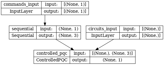
此模型採用兩個輸入:控制器的指令,以及控制器嘗試修正的輸入電路輸出。
2.4 資料集
模型嘗試針對每個指令輸出 \(\hat{Z}\) 的正確量測值。指令和正確值定義如下。
# The command input values to the classical NN.
commands = np.array([[0], [1]], dtype=np.float32)

# The desired Z expectation value at output of quantum circuit.
expected_outputs = np.array([[1], [-1]], dtype=np.float32)
這不是此工作的完整訓練資料集。資料集中的每個資料點也需要輸入電路。
2.4 輸入電路定義
以下輸入電路定義模型將學習修正的隨機錯誤校正。
random_rotations = np.random.uniform(0, 2 * np.pi, 3)
noisy_preparation = cirq.Circuit(
  cirq.rx(random_rotations[0])(qubit),
  cirq.ry(random_rotations[1])(qubit),
  cirq.rz(random_rotations[2])(qubit)
)
datapoint_circuits = tfq.convert_to_tensor([
  noisy_preparation
] * 2)  # Make two copied of this circuit
每個資料點的電路都有兩個副本。
datapoint_circuits.shape
TensorShape([2])
2.5 訓練
定義輸入後,您可以測試執行 tfq 模型。
model([datapoint_circuits, commands]).numpy()
array([[-0.13725013],
       [-0.13366866]], dtype=float32)
現在執行標準訓練程序,以將這些值調整為 expected_outputs。
optimizer = tf.keras.optimizers.Adam(learning_rate=0.05)
loss = tf.keras.losses.MeanSquaredError()
model.compile(optimizer=optimizer, loss=loss)
history = model.fit(x=[datapoint_circuits, commands],
                    y=expected_outputs,
                    epochs=30,
                    verbose=0)
plt.plot(history.history['loss'])
plt.title("Learning to Control a Qubit")
plt.xlabel("Iterations")
plt.ylabel("Error in Control")
plt.show()
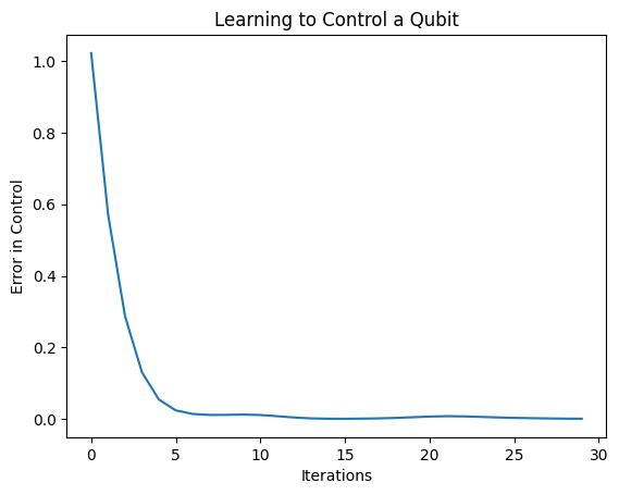
從此圖中,您可以看到神經網路已學會克服系統性錯誤校正。
2.6 驗證輸出
現在使用訓練後的模型來修正量子位元校正錯誤。搭配 Cirq
def check_error(command_values, desired_values):
  """Based on the value in `command_value` see how well you could prepare
  the full circuit to have `desired_value` when taking expectation w.r.t. Z."""
  params_to_prepare_output = controller(command_values).numpy()
  full_circuit = noisy_preparation + model_circuit

  # Test how well you can prepare a state to get expectation the expectation
  # value in `desired_values`
  for index in [0, 1]:
    state = cirq_simulator.simulate(
        full_circuit,
        {s:v for (s,v) in zip(control_params, params_to_prepare_output[index])}
    ).final_state_vector
    expt = cirq.Z(qubit).expectation_from_state_vector(state, {qubit: 0}).real
    print(f'For a desired output (expectation) of {desired_values[index]} with'
          f' noisy preparation, the controller\nnetwork found the following '
          f'values for theta: {params_to_prepare_output[index]}\nWhich gives an'
          f' actual expectation of: {expt}\n')


check_error(commands, expected_outputs)
For a desired output (expectation) of [1.] with noisy preparation, the controller
network found the following values for theta: [ 1.1249783  1.6464207 -2.502687 ]
Which gives an actual expectation of: 0.9762285351753235

For a desired output (expectation) of [-1.] with noisy preparation, the controller
network found the following values for theta: [-1.0330195 -1.6024671  0.2864415]
Which gives an actual expectation of: -0.9853028655052185
訓練期間的損失函數值大致說明模型學習狀況。損失越低,上方儲存格中的期望值就越接近 desired_values。如果您不那麼關心參數值,您可以隨時使用 tfq 檢查上方的輸出
model([datapoint_circuits, commands])
<tf.Tensor: shape=(2, 1), dtype=float32, numpy=
array([[ 0.9762286],
       [-0.9853029]], dtype=float32)>
3 學習準備不同運算符的特徵態
對應於 1 和 0 的 \(\pm \hat{Z}\) 特徵態選擇是任意的。您可能同樣希望 1 對應於 \(+ \hat{Z}\) 特徵態,而 0 對應於 \(-\hat{X}\) 特徵態。達成此目的的一種方法是為每個指令指定不同的量測運算符,如下圖所示

這需要使用 tfq.layers.Expectation。現在您的輸入已擴增為包含三個物件:電路、指令和運算符。輸出仍然是期望值。
3.1 新模型定義
讓我們來看看完成此工作的模型
# Define inputs.
commands_input = tf.keras.layers.Input(shape=(1),
                                       dtype=tf.dtypes.float32,
                                       name='commands_input')
circuits_input = tf.keras.Input(shape=(),
                                # The circuit-tensor has dtype `tf.string`
                                dtype=tf.dtypes.string,
                                name='circuits_input')
operators_input = tf.keras.Input(shape=(1,),
                                 dtype=tf.dtypes.string,
                                 name='operators_input')
以下是控制器網路
# Define classical NN.
controller = tf.keras.Sequential([
    tf.keras.layers.Dense(10, activation='elu'),
    tf.keras.layers.Dense(3)
])
使用 tfq 將電路和控制器組合成單一 keras.Model
dense_2 = controller(commands_input)

# Since you aren't using a PQC or ControlledPQC you must append
# your model circuit onto the datapoint circuit tensor manually.
full_circuit = tfq.layers.AddCircuit()(circuits_input, append=model_circuit)
expectation_output = tfq.layers.Expectation()(full_circuit,
                                              symbol_names=control_params,
                                              symbol_values=dense_2,
                                              operators=operators_input)

# Contruct your Keras model.
two_axis_control_model = tf.keras.Model(
    inputs=[circuits_input, commands_input, operators_input],
    outputs=[expectation_output])
3.2 資料集
現在您也將納入您想要針對提供給 model_circuit 的每個資料點量測的運算符
# The operators to measure, for each command.
operator_data = tfq.convert_to_tensor([[cirq.X(qubit)], [cirq.Z(qubit)]])

# The command input values to the classical NN.
commands = np.array([[0], [1]], dtype=np.float32)

# The desired expectation value at output of quantum circuit.
expected_outputs = np.array([[1], [-1]], dtype=np.float32)
3.3 訓練
現在您已具備新的輸入和輸出,您可以再次使用 keras 進行訓練。
optimizer = tf.keras.optimizers.Adam(learning_rate=0.05)
loss = tf.keras.losses.MeanSquaredError()

two_axis_control_model.compile(optimizer=optimizer, loss=loss)

history = two_axis_control_model.fit(
    x=[datapoint_circuits, commands, operator_data],
    y=expected_outputs,
    epochs=30,
    verbose=1)
Epoch 1/30
1/1 [==============================] - 0s 482ms/step - loss: 1.0518
Epoch 2/30
1/1 [==============================] - 0s 4ms/step - loss: 0.6841
Epoch 3/30
1/1 [==============================] - 0s 4ms/step - loss: 0.4386
Epoch 4/30
1/1 [==============================] - 0s 4ms/step - loss: 0.2500
Epoch 5/30
1/1 [==============================] - 0s 4ms/step - loss: 0.1179
Epoch 6/30
1/1 [==============================] - 0s 4ms/step - loss: 0.0456
Epoch 7/30
1/1 [==============================] - 0s 4ms/step - loss: 0.0172
Epoch 8/30
1/1 [==============================] - 0s 4ms/step - loss: 0.0077
Epoch 9/30
1/1 [==============================] - 0s 4ms/step - loss: 0.0035
Epoch 10/30
1/1 [==============================] - 0s 4ms/step - loss: 0.0026
Epoch 11/30
1/1 [==============================] - 0s 4ms/step - loss: 0.0060
Epoch 12/30
1/1 [==============================] - 0s 4ms/step - loss: 0.0142
Epoch 13/30
1/1 [==============================] - 0s 4ms/step - loss: 0.0256
Epoch 14/30
1/1 [==============================] - 0s 4ms/step - loss: 0.0361
Epoch 15/30
1/1 [==============================] - 0s 4ms/step - loss: 0.0430
Epoch 16/30
1/1 [==============================] - 0s 4ms/step - loss: 0.0437
Epoch 17/30
1/1 [==============================] - 0s 4ms/step - loss: 0.0359
Epoch 18/30
1/1 [==============================] - 0s 4ms/step - loss: 0.0244
Epoch 19/30
1/1 [==============================] - 0s 4ms/step - loss: 0.0146
Epoch 20/30
1/1 [==============================] - 0s 4ms/step - loss: 0.0079
Epoch 21/30
1/1 [==============================] - 0s 4ms/step - loss: 0.0038
Epoch 22/30
1/1 [==============================] - 0s 4ms/step - loss: 0.0016
Epoch 23/30
1/1 [==============================] - 0s 4ms/step - loss: 6.0264e-04
Epoch 24/30
1/1 [==============================] - 0s 4ms/step - loss: 1.8856e-04
Epoch 25/30
1/1 [==============================] - 0s 4ms/step - loss: 5.0837e-05
Epoch 26/30
1/1 [==============================] - 0s 4ms/step - loss: 1.5398e-05
Epoch 27/30
1/1 [==============================] - 0s 4ms/step - loss: 1.2333e-05
Epoch 28/30
1/1 [==============================] - 0s 4ms/step - loss: 2.5812e-05
Epoch 29/30
1/1 [==============================] - 0s 4ms/step - loss: 6.2401e-05
Epoch 30/30
1/1 [==============================] - 0s 4ms/step - loss: 1.3390e-04
plt.plot(history.history['loss'])
plt.title("Learning to Control a Qubit")
plt.xlabel("Iterations")
plt.ylabel("Error in Control")
plt.show()
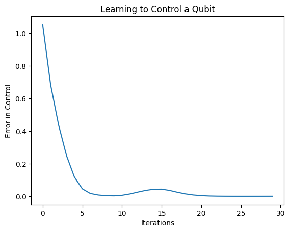
損失函數已降至零。
controller 可作為獨立模型使用。呼叫控制器,並檢查它對每個指令訊號的回應。需要一些工作才能正確地將這些輸出與 random_rotations 的內容進行比較。
controller.predict(np.array([0,1]))
1/1 [==============================] - 0s 67ms/step
array([[ 1.6641312 , -0.06845868, -0.00440133],
       [ 0.59975535, -1.9673042 ,  1.7837791 ]], dtype=float32)