
|
|
|
 在 GitHub 上檢視原始碼 在 GitHub 上檢視原始碼
|
|
本教學課程探討量子電路期望值的梯度計算演算法。
計算量子電路中特定可觀測值的期望值梯度是一個複雜的過程。可觀測值的期望值不像傳統機器學習轉換 (例如易於寫出的解析梯度公式的矩陣乘法或向量加法) 那樣,具有總是易於寫出的解析梯度公式。因此,有不同的量子梯度計算方法在不同的情境中會派上用場。本教學課程將比較和對照兩種不同的微分機制。
設定
pip install tensorflow==2.15.0
安裝 TensorFlow Quantum
pip install tensorflow-quantum==0.7.3
# Update package resources to account for version changes.
import importlib, pkg_resources
importlib.reload(pkg_resources)
/tmpfs/tmp/ipykernel_13801/1875984233.py:2: DeprecationWarning: pkg_resources is deprecated as an API. See https://setuptools.pypa.io/en/latest/pkg_resources.html
  import importlib, pkg_resources
<module 'pkg_resources' from '/tmpfs/src/tf_docs_env/lib/python3.9/site-packages/pkg_resources/__init__.py'>
現在匯入 TensorFlow 和模組依附元件
import tensorflow as tf
import tensorflow_quantum as tfq

import cirq
import sympy
import numpy as np

# visualization tools
%matplotlib inline
import matplotlib.pyplot as plt
from cirq.contrib.svg import SVGCircuit
2024-05-18 11:25:27.526147: E external/local_xla/xla/stream_executor/cuda/cuda_dnn.cc:9261] Unable to register cuDNN factory: Attempting to register factory for plugin cuDNN when one has already been registered
2024-05-18 11:25:27.526190: E external/local_xla/xla/stream_executor/cuda/cuda_fft.cc:607] Unable to register cuFFT factory: Attempting to register factory for plugin cuFFT when one has already been registered
2024-05-18 11:25:27.527683: E external/local_xla/xla/stream_executor/cuda/cuda_blas.cc:1515] Unable to register cuBLAS factory: Attempting to register factory for plugin cuBLAS when one has already been registered
2024-05-18 11:25:30.854843: E external/local_xla/xla/stream_executor/cuda/cuda_driver.cc:274] failed call to cuInit: CUDA_ERROR_NO_DEVICE: no CUDA-capable device is detected
1. 預備知識
讓我們更具體地說明量子電路梯度計算的概念。假設您有一個像這樣的參數化電路
qubit = cirq.GridQubit(0, 0)
my_circuit = cirq.Circuit(cirq.Y(qubit)**sympy.Symbol('alpha'))
SVGCircuit(my_circuit)
findfont: Font family 'Arial' not found.
findfont: Font family 'Arial' not found.

以及一個可觀測值
pauli_x = cirq.X(qubit)
pauli_x
cirq.X(cirq.GridQubit(0, 0))
觀察此運算子,您會知道 \(⟨Y(\alpha)| X | Y(\alpha)⟩ = \sin(\pi \alpha)\)
def my_expectation(op, alpha):
    """Compute ⟨Y(alpha)| `op` | Y(alpha)⟩"""
    params = {'alpha': alpha}
    sim = cirq.Simulator()
    final_state_vector = sim.simulate(my_circuit, params).final_state_vector
    return op.expectation_from_state_vector(final_state_vector, {qubit: 0}).real


my_alpha = 0.3
print("Expectation=", my_expectation(pauli_x, my_alpha))
print("Sin Formula=", np.sin(np.pi * my_alpha))
Expectation= 0.80901700258255
Sin Formula= 0.8090169943749475
如果您定義 \(f_{1}(\alpha) = ⟨Y(\alpha)| X | Y(\alpha)⟩\),則 \(f_{1}^{'}(\alpha) = \pi \cos(\pi \alpha)\)。讓我們檢查一下
def my_grad(obs, alpha, eps=0.01):
    grad = 0
    f_x = my_expectation(obs, alpha)
    f_x_prime = my_expectation(obs, alpha + eps)
    return ((f_x_prime - f_x) / eps).real


print('Finite difference:', my_grad(pauli_x, my_alpha))
print('Cosine formula:   ', np.pi * np.cos(np.pi * my_alpha))
Finite difference: 1.8063604831695557
Cosine formula:    1.8465818304904567
2. 微分器的需求
對於較大的電路,您不一定總是很幸運能有一個精確計算給定量子電路梯度的公式。在簡單公式不足以計算梯度的情況下,tfq.differentiators.Differentiator 類別可讓您定義用於計算電路梯度的演算法。例如,您可以使用以下程式碼在 TensorFlow Quantum (TFQ) 中重新建立上述範例
expectation_calculation = tfq.layers.Expectation(
    differentiator=tfq.differentiators.ForwardDifference(grid_spacing=0.01))

expectation_calculation(my_circuit,
                        operators=pauli_x,
                        symbol_names=['alpha'],
                        symbol_values=[[my_alpha]])
<tf.Tensor: shape=(1, 1), dtype=float32, numpy=array([[0.80901706]], dtype=float32)>
不過,如果您切換為根據取樣 (真實裝置上會發生的情況) 估計期望值,則值可能會稍微改變。這表示您現在會有不完美的估計值
sampled_expectation_calculation = tfq.layers.SampledExpectation(
    differentiator=tfq.differentiators.ForwardDifference(grid_spacing=0.01))

sampled_expectation_calculation(my_circuit,
                                operators=pauli_x,
                                repetitions=500,
                                symbol_names=['alpha'],
                                symbol_values=[[my_alpha]])
<tf.Tensor: shape=(1, 1), dtype=float32, numpy=array([[0.832]], dtype=float32)>
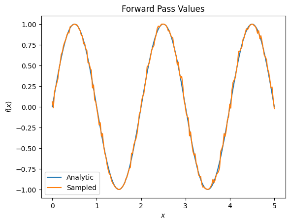
當涉及到梯度時,這可能會迅速累積成嚴重的準確性問題
# Make input_points = [batch_size, 1] array.
input_points = np.linspace(0, 5, 200)[:, np.newaxis].astype(np.float32)
exact_outputs = expectation_calculation(my_circuit,
                                        operators=pauli_x,
                                        symbol_names=['alpha'],
                                        symbol_values=input_points)
imperfect_outputs = sampled_expectation_calculation(my_circuit,
                                                    operators=pauli_x,
                                                    repetitions=500,
                                                    symbol_names=['alpha'],
                                                    symbol_values=input_points)
plt.title('Forward Pass Values')
plt.xlabel('$x$')
plt.ylabel('$f(x)$')
plt.plot(input_points, exact_outputs, label='Analytic')
plt.plot(input_points, imperfect_outputs, label='Sampled')
plt.legend()
<matplotlib.legend.Legend at 0x7f3c740e74c0>
# Gradients are a much different story.
values_tensor = tf.convert_to_tensor(input_points)

with tf.GradientTape() as g:
    g.watch(values_tensor)
    exact_outputs = expectation_calculation(my_circuit,
                                            operators=pauli_x,
                                            symbol_names=['alpha'],
                                            symbol_values=values_tensor)
analytic_finite_diff_gradients = g.gradient(exact_outputs, values_tensor)

with tf.GradientTape() as g:
    g.watch(values_tensor)
    imperfect_outputs = sampled_expectation_calculation(
        my_circuit,
        operators=pauli_x,
        repetitions=500,
        symbol_names=['alpha'],
        symbol_values=values_tensor)
sampled_finite_diff_gradients = g.gradient(imperfect_outputs, values_tensor)

plt.title('Gradient Values')
plt.xlabel('$x$')
plt.ylabel('$f^{\'}(x)$')
plt.plot(input_points, analytic_finite_diff_gradients, label='Analytic')
plt.plot(input_points, sampled_finite_diff_gradients, label='Sampled')
plt.legend()
<matplotlib.legend.Legend at 0x7f3b6c627fd0>
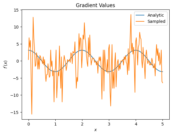
在這裡您可以看到,雖然有限差分公式在分析案例中可以快速計算梯度本身,但當涉及到基於取樣的方法時,雜訊卻過多。必須使用更謹慎的技術來確保可以計算出良好的梯度。接下來,您將看到一種速度較慢的技術,這種技術不太適合分析期望值梯度計算,但在真實世界的基於樣本的案例中表現得更好
# A smarter differentiation scheme.
gradient_safe_sampled_expectation = tfq.layers.SampledExpectation(
    differentiator=tfq.differentiators.ParameterShift())

with tf.GradientTape() as g:
    g.watch(values_tensor)
    imperfect_outputs = gradient_safe_sampled_expectation(
        my_circuit,
        operators=pauli_x,
        repetitions=500,
        symbol_names=['alpha'],
        symbol_values=values_tensor)

sampled_param_shift_gradients = g.gradient(imperfect_outputs, values_tensor)

plt.title('Gradient Values')
plt.xlabel('$x$')
plt.ylabel('$f^{\'}(x)$')
plt.plot(input_points, analytic_finite_diff_gradients, label='Analytic')
plt.plot(input_points, sampled_param_shift_gradients, label='Sampled')
plt.legend()
<matplotlib.legend.Legend at 0x7f3b6c557400>
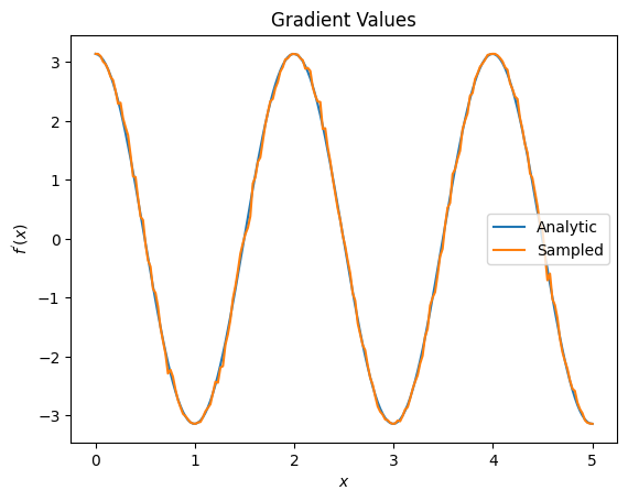
從以上內容可以看出,某些微分器最適合用於特定的研究情境。一般而言,速度較慢的基於樣本的方法對於裝置雜訊等具有強大的抗干擾能力,是在更「真實世界」的設定中測試或實作演算法的絕佳微分器。像有限差分這樣速度較快的方法非常適合用於分析計算,而且您需要更高的輸送量,但還不擔心演算法在裝置上的可行性。
3. 多個可觀測值
讓我們引入第二個可觀測值,看看 TensorFlow Quantum 如何支援單一電路的多個可觀測值。
pauli_z = cirq.Z(qubit)
pauli_z
cirq.Z(cirq.GridQubit(0, 0))
如果此可觀測值與先前的電路一起使用,則您會得到 \(f_{2}(\alpha) = ⟨Y(\alpha)| Z | Y(\alpha)⟩ = \cos(\pi \alpha)\) 和 \(f_{2}^{'}(\alpha) = -\pi \sin(\pi \alpha)\)。快速檢查一下
test_value = 0.

print('Finite difference:', my_grad(pauli_z, test_value))
print('Sin formula:      ', -np.pi * np.sin(np.pi * test_value))
Finite difference: -0.04934072494506836
Sin formula:       -0.0
完全符合 (非常接近)。
現在,如果您定義 \(g(\alpha) = f_{1}(\alpha) + f_{2}(\alpha)\),則 \(g'(\alpha) = f_{1}^{'}(\alpha) + f^{'}_{2}(\alpha)\)。在 TensorFlow Quantum 中定義多個可觀測值以與電路一起使用,相當於在 \(g\) 中新增更多項。
這表示電路中特定符號的梯度等於針對該符號應用於該電路的每個可觀測值的梯度總和。這與 TensorFlow 梯度運算和反向傳播相容 (在反向傳播中,您會提供所有可觀測值的梯度總和作為特定符號的梯度)。
sum_of_outputs = tfq.layers.Expectation(
    differentiator=tfq.differentiators.ForwardDifference(grid_spacing=0.01))

sum_of_outputs(my_circuit,
               operators=[pauli_x, pauli_z],
               symbol_names=['alpha'],
               symbol_values=[[test_value]])
<tf.Tensor: shape=(1, 2), dtype=float32, numpy=array([[1.9106855e-15, 1.0000000e+00]], dtype=float32)>
在這裡您可以看到,第一個項目是相對於 Pauli X 的期望值,第二個項目是相對於 Pauli Z 的期望值。現在當您取梯度時
test_value_tensor = tf.convert_to_tensor([[test_value]])

with tf.GradientTape() as g:
    g.watch(test_value_tensor)
    outputs = sum_of_outputs(my_circuit,
                             operators=[pauli_x, pauli_z],
                             symbol_names=['alpha'],
                             symbol_values=test_value_tensor)

sum_of_gradients = g.gradient(outputs, test_value_tensor)

print(my_grad(pauli_x, test_value) + my_grad(pauli_z, test_value))
print(sum_of_gradients.numpy())
3.0917350202798843
[[3.0917213]]
在這裡,您已驗證每個可觀測值的梯度總和確實是 \(\alpha\) 的梯度。所有 TensorFlow Quantum 微分器都支援此行為,並且在與 TensorFlow 的其餘部分相容方面發揮關鍵作用。
4. 進階用法
TensorFlow Quantum 內的所有微分器都是 tfq.differentiators.Differentiator 的子類別。若要實作微分器,使用者必須實作兩個介面之一。標準做法是實作 get_gradient_circuits,這會告知基礎類別要測量哪些電路才能取得梯度估計值。或者,您可以覆寫 differentiate_analytic 和 differentiate_sampled;tfq.differentiators.Adjoint 類別採用這種方法。
以下範例使用 TensorFlow Quantum 實作電路的梯度。您將使用參數平移的小範例。
回想一下您在上面定義的電路 \(|\alpha⟩ = Y^{\alpha}|0⟩\)。與之前一樣,您可以將函數定義為此電路相對於 \(X\) 可觀測值的期望值,\(f(\alpha) = ⟨\alpha|X|\alpha⟩\)。使用參數平移規則,對於此電路,您可以找到導數為
\[\frac{\partial}{\partial \alpha} f(\alpha) = \frac{\pi}{2} f\left(\alpha + \frac{1}{2}\right) - \frac{ \pi}{2} f\left(\alpha - \frac{1}{2}\right)\]
get_gradient_circuits 函數會傳回此導數的組件。
class MyDifferentiator(tfq.differentiators.Differentiator):
    """A Toy differentiator for <Y^alpha | X |Y^alpha>."""

    def __init__(self):
        pass

    def get_gradient_circuits(self, programs, symbol_names, symbol_values):
        """Return circuits to compute gradients for given forward pass circuits.

        Every gradient on a quantum computer can be computed via measurements
        of transformed quantum circuits.  Here, you implement a custom gradient
        for a specific circuit.  For a real differentiator, you will need to
        implement this function in a more general way.  See the differentiator
        implementations in the TFQ library for examples.
        """

        # The two terms in the derivative are the same circuit...
        batch_programs = tf.stack([programs, programs], axis=1)

        # ... with shifted parameter values.
        shift = tf.constant(1/2)
        forward = symbol_values + shift
        backward = symbol_values - shift
        batch_symbol_values = tf.stack([forward, backward], axis=1)

        # Weights are the coefficients of the terms in the derivative.
        num_program_copies = tf.shape(batch_programs)[0]
        batch_weights = tf.tile(tf.constant([[[np.pi/2, -np.pi/2]]]),
                                [num_program_copies, 1, 1])

        # The index map simply says which weights go with which circuits.
        batch_mapper = tf.tile(
            tf.constant([[[0, 1]]]), [num_program_copies, 1, 1])

        return (batch_programs, symbol_names, batch_symbol_values,
                batch_weights, batch_mapper)
Differentiator 基礎類別會使用從 get_gradient_circuits 傳回的組件來計算導數,就像您在上面看到的參數平移公式一樣。這個新的微分器現在可以與現有的 tfq.layer 物件搭配使用
custom_dif = MyDifferentiator()
custom_grad_expectation = tfq.layers.Expectation(differentiator=custom_dif)

# Now let's get the gradients with finite diff.
with tf.GradientTape() as g:
    g.watch(values_tensor)
    exact_outputs = expectation_calculation(my_circuit,
                                            operators=[pauli_x],
                                            symbol_names=['alpha'],
                                            symbol_values=values_tensor)

analytic_finite_diff_gradients = g.gradient(exact_outputs, values_tensor)

# Now let's get the gradients with custom diff.
with tf.GradientTape() as g:
    g.watch(values_tensor)
    my_outputs = custom_grad_expectation(my_circuit,
                                         operators=[pauli_x],
                                         symbol_names=['alpha'],
                                         symbol_values=values_tensor)

my_gradients = g.gradient(my_outputs, values_tensor)

plt.subplot(1, 2, 1)
plt.title('Exact Gradient')
plt.plot(input_points, analytic_finite_diff_gradients.numpy())
plt.xlabel('x')
plt.ylabel('f(x)')
plt.subplot(1, 2, 2)
plt.title('My Gradient')
plt.plot(input_points, my_gradients.numpy())
plt.xlabel('x')
Text(0.5, 0, 'x')
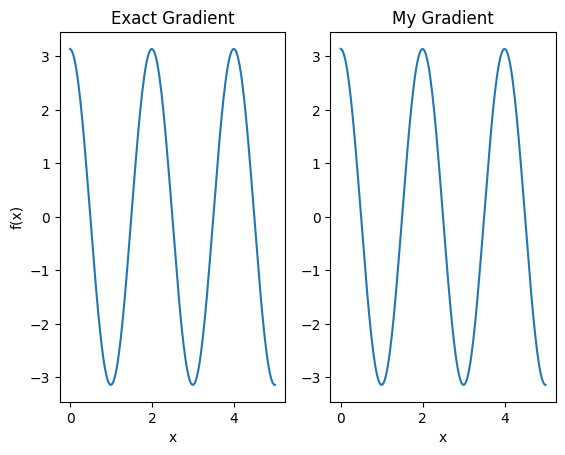
這個新的微分器現在可以用於產生可微分的運算。
# Create a noisy sample based expectation op.
expectation_sampled = tfq.get_sampled_expectation_op(
    cirq.DensityMatrixSimulator(noise=cirq.depolarize(0.01)))

# Make it differentiable with your differentiator:
# Remember to refresh the differentiator before attaching the new op
custom_dif.refresh()
differentiable_op = custom_dif.generate_differentiable_op(
    sampled_op=expectation_sampled)

# Prep op inputs.
circuit_tensor = tfq.convert_to_tensor([my_circuit])
op_tensor = tfq.convert_to_tensor([[pauli_x]])
single_value = tf.convert_to_tensor([[my_alpha]])
num_samples_tensor = tf.convert_to_tensor([[5000]])

with tf.GradientTape() as g:
    g.watch(single_value)
    forward_output = differentiable_op(circuit_tensor, ['alpha'], single_value,
                                       op_tensor, num_samples_tensor)

my_gradients = g.gradient(forward_output, single_value)

print('---TFQ---')
print('Foward:  ', forward_output.numpy())
print('Gradient:', my_gradients.numpy())
print('---Original---')
print('Forward: ', my_expectation(pauli_x, my_alpha))
print('Gradient:', my_grad(pauli_x, my_alpha))
---TFQ---
Foward:   [[0.7816]]
Gradient: [[1.7919645]]
---Original---
Forward:  0.80901700258255
Gradient: 1.8063604831695557