在 TensorFlow.org 上檢視

在 Google Colab 中執行

在 GitHub 上檢視原始碼

下載筆記本

總覽

本教學課程示範如何使用 TensorFlow Lattice (TFL) 程式庫訓練*負責任*的模型，且模型不會違反某些*合乎倫理*或*公平*的假設。我們將特別著重於使用單調性限制來避免對特定屬性進行*不公平的懲罰*。本教學課程包含 Serena Wang 和 Maya Gupta 於 AISTATS 2020 發表的論文 Deontological Ethics By Monotonicity Shape Constraints 中的實驗示範。

我們將在公開資料集上使用 TFL 預製模型，但請注意，本教學課程中的所有內容也可以使用從 TFL Keras 層建構的模型來完成。

繼續之前，請確保您的執行階段已安裝所有必要的套件 (如下方程式碼儲存格中匯入的套件)。

設定

安裝 TF Lattice 套件

pip install --pre -U tensorflow tf-keras tensorflow-lattice tensorflow_decision_forests seaborn pydot graphviz

匯入必要的套件

import tensorflow as tf
import tensorflow_lattice as tfl
import tensorflow_decision_forests as tfdf

import logging
import matplotlib.pyplot as plt
import numpy as np
import os
import pandas as pd
import seaborn as sns
from sklearn.model_selection import train_test_split
import sys
import tempfile
logging.disable(sys.maxsize)

# Use Keras 2.
version_fn = getattr(tf.keras, "version", None)
if version_fn and version_fn().startswith("3."):
  import tf_keras as keras
else:
  keras = tf.keras

本教學課程中使用的預設值

# Default number of training epochs, batch sizes and learning rate.
NUM_EPOCHS = 256
BATCH_SIZE = 256
LEARNING_RATES = 0.01
# Directory containing dataset files.
DATA_DIR = 'https://raw.githubusercontent.com/serenalwang/shape_constraints_for_ethics/master'

個案研究 1：法學院入學許可

在本教學課程的第一部分，我們將考量使用法學院入學委員會 (LSAC) 的法學院入學許可資料集的個案研究。我們將訓練分類器，使用兩個特徵 (學生的 LSAT 分數和大學 GPA) 來預測學生是否會通過律師考試。

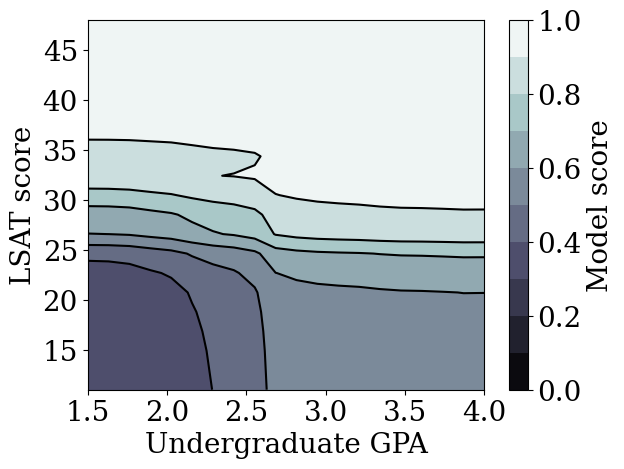
假設分類器的分數用於引導法學院入學許可或獎學金。根據以績效為基礎的社會規範，我們預期 GPA 較高和 LSAT 分數較高的學生應從分類器獲得較高的分數。但是，我們將觀察到模型很容易違反這些直覺規範，有時會因為人們的 GPA 或 LSAT 分數較高而懲罰他們。

為了解決這個*不公平懲罰*問題，我們可以施加單調性限制，使模型永遠不會懲罰較高的 GPA 或較高的 LSAT 分數，在所有其他條件相同的情況下。在本教學課程中，我們將說明如何使用 TFL 施加這些單調性限制。

載入法學院資料

# Load data file.
law_file_name = 'lsac.csv'
law_file_path = os.path.join(DATA_DIR, law_file_name)
raw_law_df = pd.read_csv(law_file_path, delimiter=',')

預先處理資料集

# Define label column name.
LAW_LABEL = 'pass_bar'

def preprocess_law_data(input_df):
  # Drop rows with where the label or features of interest are missing.
  output_df = input_df[~input_df[LAW_LABEL].isna() & ~input_df['ugpa'].isna() &
                       (input_df['ugpa'] > 0) & ~input_df['lsat'].isna()]
  return output_df


law_df = preprocess_law_data(raw_law_df)

將資料分割為訓練/驗證/測試集

def split_dataset(input_df, random_state=888):
  """Splits an input dataset into train, val, and test sets."""
  train_df, test_val_df = train_test_split(
      input_df, test_size=0.3, random_state=random_state
  )
  val_df, test_df = train_test_split(
      test_val_df, test_size=0.66, random_state=random_state
  )
  return train_df, val_df, test_df


dataframes = {}
datasets = {}

(dataframes['law_train'], dataframes['law_val'], dataframes['law_test']) = (
    split_dataset(law_df)
)

for df_name, df in dataframes.items():
  datasets[df_name] = tf.data.Dataset.from_tensor_slices(
      ((df[['ugpa']], df[['lsat']]), df[['pass_bar']])
  ).batch(BATCH_SIZE)

2024-03-27 11:20:52.644317: E external/local_xla/xla/stream_executor/cuda/cuda_driver.cc:282] failed call to cuInit: CUDA_ERROR_NO_DEVICE: no CUDA-capable device is detected

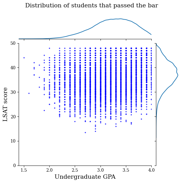
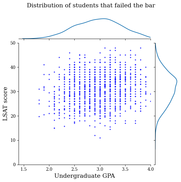
視覺化資料分佈

首先，我們將視覺化資料的分佈。我們將繪製所有通過律師考試的學生以及所有未通過律師考試的學生的 GPA 和 LSAT 分數。

def plot_dataset_contour(input_df, title):
  plt.rcParams['font.family'] = ['serif']
  g = sns.jointplot(
      x='ugpa',
      y='lsat',
      data=input_df,
      kind='kde',
      xlim=[1.4, 4],
      ylim=[0, 50])
  g.plot_joint(plt.scatter, c='b', s=10, linewidth=1, marker='+')
  g.ax_joint.collections[0].set_alpha(0)
  g.set_axis_labels('Undergraduate GPA', 'LSAT score', fontsize=14)
  g.fig.suptitle(title, fontsize=14)
  # Adust plot so that the title fits.
  plt.subplots_adjust(top=0.9)
  plt.show()

law_df_pos = law_df[law_df[LAW_LABEL] == 1]
plot_dataset_contour(
    law_df_pos, title='Distribution of students that passed the bar')
law_df_neg = law_df[law_df[LAW_LABEL] == 0]
plot_dataset_contour(
    law_df_neg, title='Distribution of students that failed the bar')

訓練校正晶格模型以預測律師考試通過情況

接下來，我們將從 TFL 訓練*校正晶格模型*，以預測學生是否會通過律師考試。兩個輸入特徵將是 LSAT 分數和大學 GPA，而訓練標籤將是學生是否通過律師考試。

我們先訓練一個沒有任何限制的校正晶格模型。然後，我們將訓練一個具有單調性限制的校正晶格模型，並觀察模型輸出和準確度的差異。

用於視覺化已訓練模型輸出的輔助函式

def plot_model_contour(model, from_logits=False, num_keypoints=20):
  x = np.linspace(min(law_df['ugpa']), max(law_df['ugpa']), num_keypoints)
  y = np.linspace(min(law_df['lsat']), max(law_df['lsat']), num_keypoints)

  x_grid, y_grid = np.meshgrid(x, y)

  positions = np.vstack([x_grid.ravel(), y_grid.ravel()])
  plot_df = pd.DataFrame(positions.T, columns=['ugpa', 'lsat'])
  plot_df[LAW_LABEL] = np.ones(len(plot_df))
  predictions = model.predict((plot_df[['ugpa']], plot_df[['lsat']]))
  if from_logits:
    predictions = tf.math.sigmoid(predictions)
  grid_predictions = np.reshape(predictions, x_grid.shape)

  plt.rcParams['font.family'] = ['serif']
  plt.contour(
      x_grid,
      y_grid,
      grid_predictions,
      colors=('k',),
      levels=np.linspace(0, 1, 11),
  )
  plt.contourf(
      x_grid,
      y_grid,
      grid_predictions,
      cmap=plt.cm.bone,
      levels=np.linspace(0, 1, 11),
  )
  plt.xticks(fontsize=20)
  plt.yticks(fontsize=20)

  cbar = plt.colorbar()
  cbar.ax.set_ylabel('Model score', fontsize=20)
  cbar.ax.tick_params(labelsize=20)

  plt.xlabel('Undergraduate GPA', fontsize=20)
  plt.ylabel('LSAT score', fontsize=20)

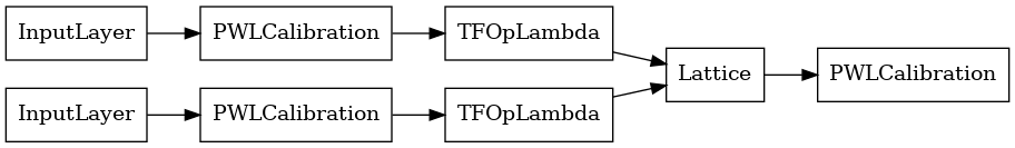
訓練未受限制 (非單調) 的校正晶格模型

我們使用 'CalibratedLatticeConfig 建立 TFL 預製模型。此模型是具有輸出校正的校正晶格模型。

model_config = tfl.configs.CalibratedLatticeConfig(
    feature_configs=[
        tfl.configs.FeatureConfig(
            name='ugpa',
            lattice_size=3,
            pwl_calibration_num_keypoints=16,
            monotonicity=0,
            pwl_calibration_always_monotonic=False,
        ),
        tfl.configs.FeatureConfig(
            name='lsat',
            lattice_size=3,
            pwl_calibration_num_keypoints=16,
            monotonicity=0,
            pwl_calibration_always_monotonic=False,
        ),
    ],
    output_calibration=True,
    output_initialization=np.linspace(-2, 2, num=8),
)

我們使用 premade_lib API 計算並填入特徵配置中的特徵分位數。

feature_keypoints = tfl.premade_lib.compute_feature_keypoints(
    feature_configs=model_config.feature_configs,
    features=dataframes['law_train'][['ugpa', 'lsat', 'pass_bar']],
)
tfl.premade_lib.set_feature_keypoints(
    feature_configs=model_config.feature_configs,
    feature_keypoints=feature_keypoints,
    add_missing_feature_configs=False,
)

nomon_lattice_model = tfl.premade.CalibratedLattice(model_config=model_config)
keras.utils.plot_model(
    nomon_lattice_model, expand_nested=True, show_layer_names=False, rankdir="LR"
)

nomon_lattice_model.compile(
    loss=keras.losses.BinaryCrossentropy(from_logits=True),
    metrics=[
        keras.metrics.BinaryAccuracy(name='accuracy'),
    ],
    optimizer=keras.optimizers.Adam(LEARNING_RATES),
)
nomon_lattice_model.fit(datasets['law_train'], epochs=NUM_EPOCHS, verbose=0)

train_acc = nomon_lattice_model.evaluate(datasets['law_train'])[1]
val_acc = nomon_lattice_model.evaluate(datasets['law_val'])[1]
test_acc = nomon_lattice_model.evaluate(datasets['law_test'])[1]
print(
    'accuracies for train: %f, val: %f, test: %f'
    % (train_acc, val_acc, test_acc)
)

63/63 [==============================] - 1s 1ms/step - loss: 0.1727 - accuracy: 0.9460
10/10 [==============================] - 0s 2ms/step - loss: 0.1877 - accuracy: 0.9390
18/18 [==============================] - 0s 1ms/step - loss: 0.1672 - accuracy: 0.9480
accuracies for train: 0.945995, val: 0.939003, test: 0.948020

plot_model_contour(nomon_lattice_model, from_logits=True)

13/13 [==============================] - 0s 1ms/step

訓練單調校正晶格模型

我們可以透過在特徵配置中設定單調性限制來取得單調模型。

model_config.feature_configs[0].monotonicity = 1
model_config.feature_configs[1].monotonicity = 1

mon_lattice_model = tfl.premade.CalibratedLattice(model_config=model_config)

mon_lattice_model.compile(
    loss=keras.losses.BinaryCrossentropy(from_logits=True),
    metrics=[
        keras.metrics.BinaryAccuracy(name='accuracy'),
    ],
    optimizer=keras.optimizers.Adam(LEARNING_RATES),
)
mon_lattice_model.fit(datasets['law_train'], epochs=NUM_EPOCHS, verbose=0)

train_acc = mon_lattice_model.evaluate(datasets['law_train'])[1]
val_acc = mon_lattice_model.evaluate(datasets['law_val'])[1]
test_acc = mon_lattice_model.evaluate(datasets['law_test'])[1]
print(
    'accuracies for train: %f, val: %f, test: %f'
    % (train_acc, val_acc, test_acc)
)

63/63 [==============================] - 0s 1ms/step - loss: 0.1712 - accuracy: 0.9463
10/10 [==============================] - 0s 2ms/step - loss: 0.1869 - accuracy: 0.9403
18/18 [==============================] - 0s 2ms/step - loss: 0.1654 - accuracy: 0.9487
accuracies for train: 0.946308, val: 0.940292, test: 0.948684

plot_model_contour(mon_lattice_model, from_logits=True)

13/13 [==============================] - 0s 1ms/step

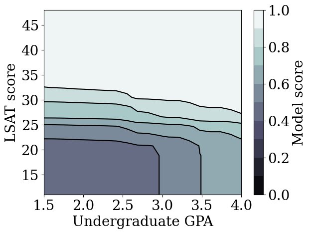
我們示範了可以訓練 TFL 校正晶格模型在 LSAT 分數和 GPA 中都具有單調性，而不會在準確度方面做出太大的犧牲。

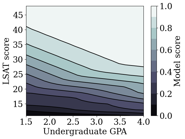
訓練其他未受限制的模型

校正晶格模型與其他類型的模型 (例如深度神經網路 (DNN) 或梯度提升樹 (GBT)) 相比如何？DNN 和 GBT 似乎具有合理的公平輸出嗎？為了回答這個問題，我們接下來將訓練一個未受限制的 DNN 和 GBT。事實上，我們將觀察到 DNN 和 GBT 都很容易違反 LSAT 分數和大學 GPA 的單調性。

訓練未受限制的深度神經網路 (DNN) 模型

架構先前已最佳化，以實現高驗證準確度。

keras.utils.set_random_seed(42)
inputs = [
    keras.Input(shape=(1,), dtype=tf.float32),
    keras.Input(shape=(1), dtype=tf.float32),
]
inputs_flat = keras.layers.Concatenate()(inputs)
dense_layers = keras.Sequential(
    [
        keras.layers.Dense(64, activation='relu'),
        keras.layers.Dense(32, activation='relu'),
        keras.layers.Dense(1, activation=None),
    ],
    name='dense_layers',
)
dnn_model = keras.Model(inputs=inputs, outputs=dense_layers(inputs_flat))
dnn_model.compile(
    loss=keras.losses.BinaryCrossentropy(from_logits=True),
    metrics=[keras.metrics.BinaryAccuracy(name='accuracy')],
    optimizer=keras.optimizers.Adam(LEARNING_RATES),
)
dnn_model.fit(datasets['law_train'], epochs=NUM_EPOCHS, verbose=0)

train_acc = dnn_model.evaluate(datasets['law_train'])[1]
val_acc = dnn_model.evaluate(datasets['law_val'])[1]
test_acc = dnn_model.evaluate(datasets['law_test'])[1]
print(
    'accuracies for train: %f, val: %f, test: %f'
    % (train_acc, val_acc, test_acc)
)

63/63 [==============================] - 0s 1ms/step - loss: 0.1729 - accuracy: 0.9482
10/10 [==============================] - 0s 2ms/step - loss: 0.1846 - accuracy: 0.9424
18/18 [==============================] - 0s 1ms/step - loss: 0.1658 - accuracy: 0.9505
accuracies for train: 0.948248, val: 0.942440, test: 0.950453

plot_model_contour(dnn_model, from_logits=True)

13/13 [==============================] - 0s 1ms/step

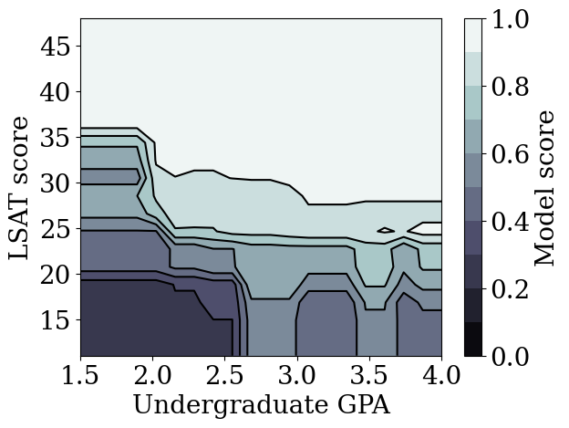
訓練未受限制的梯度提升樹 (GBT) 模型

樹狀結構先前已最佳化，以實現高驗證準確度。

tree_model = tfdf.keras.GradientBoostedTreesModel(
    exclude_non_specified_features=False,
    num_threads=1,
    num_trees=20,
    max_depth=4,
    growing_strategy='BEST_FIRST_GLOBAL',
    random_seed=42,
    temp_directory=tempfile.mkdtemp(),
)
tree_model.compile(metrics=[keras.metrics.BinaryAccuracy(name='accuracy')])
tree_model.fit(
    datasets['law_train'], validation_data=datasets['law_val'], verbose=0
)

tree_train_acc = tree_model.evaluate(datasets['law_train'], verbose=0)[1]
tree_val_acc = tree_model.evaluate(datasets['law_val'], verbose=0)[1]
tree_test_acc = tree_model.evaluate(datasets['law_test'], verbose=0)[1]
print(
    'accuracies for GBT: train: %f, val: %f, test: %f'
    % (tree_train_acc, tree_val_acc, tree_test_acc)
)

[WARNING 24-03-27 11:22:52.3549 UTC gradient_boosted_trees.cc:1840] "goss_alpha" set but "sampling_method" not equal to "GOSS".
[WARNING 24-03-27 11:22:52.3550 UTC gradient_boosted_trees.cc:1851] "goss_beta" set but "sampling_method" not equal to "GOSS".
[WARNING 24-03-27 11:22:52.3550 UTC gradient_boosted_trees.cc:1865] "selective_gradient_boosting_ratio" set but "sampling_method" not equal to "SELGB".
Num validation examples: tf.Tensor(2328, shape=(), dtype=int32)
[INFO 24-03-27 11:22:56.7210 UTC kernel.cc:1233] Loading model from path /tmpfs/tmp/tmpl7y3whz4/model/ with prefix 9539d0c1bde64ba3
[INFO 24-03-27 11:22:56.7229 UTC quick_scorer_extended.cc:911] The binary was compiled without AVX2 support, but your CPU supports it. Enable it for faster model inference.
[INFO 24-03-27 11:22:56.7230 UTC abstract_model.cc:1344] Engine "GradientBoostedTreesQuickScorerExtended" built
[INFO 24-03-27 11:22:56.7230 UTC kernel.cc:1061] Use fast generic engine
accuracies for GBT: train: 0.949625, val: 0.948024, test: 0.951559

plot_model_contour(tree_model)

13/13 [==============================] - 0s 1ms/step

個案研究 2：信用違約

我們將在本教學課程中考量的第二個個案研究是預測個人的信用違約機率。我們將使用 UCI 儲存庫的「信用卡客戶違約」資料集。此資料是從 30,000 名台灣信用卡使用者收集而來，其中包含使用者在時間範圍內是否違約付款的二元標籤。特徵包括婚姻狀況、性別、教育程度，以及使用者在 2005 年 4 月至 9 月每個月的現有帳單付款方面落後多久。

如同我們在第一個個案研究中所做的，我們再次示範使用單調性限制來避免*不公平的懲罰*：如果模型用於判斷使用者的信用評分，那麼如果使用者因為提早付款而受到懲罰，在所有其他條件相同的情況下，許多人可能會感到不公平。因此，我們套用單調性限制，以防止模型懲罰提早付款。

載入信用違約資料

# Load data file.
credit_file_name = 'credit_default.csv'
credit_file_path = os.path.join(DATA_DIR, credit_file_name)
credit_df = pd.read_csv(credit_file_path, delimiter=',')

# Define label column name.
CREDIT_LABEL = 'default'

將資料分割為訓練/驗證/測試集

dfs = {}
datasets = {}

dfs["credit_train"], dfs["credit_val"], dfs["credit_test"] = split_dataset(
    credit_df
)

for df_name, df in dfs.items():
  datasets[df_name] = tf.data.Dataset.from_tensor_slices(
      ((df[['MARRIAGE']], df[['PAY_0']]), df[['default']])
  ).batch(BATCH_SIZE)

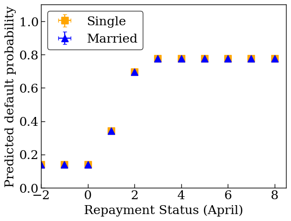
視覺化資料分佈

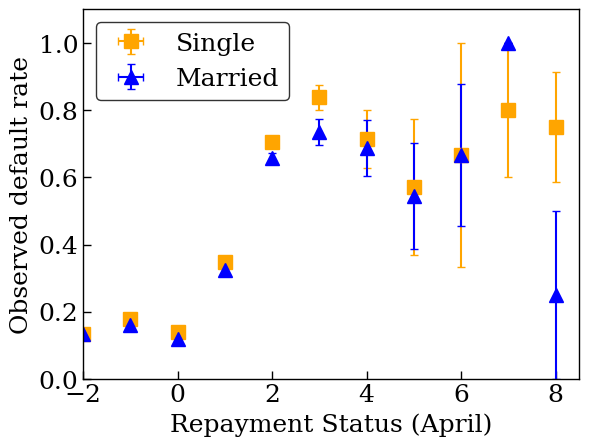
首先，我們將視覺化資料的分佈。我們將繪製具有不同婚姻狀況和還款狀況的人的觀察違約率的平均值和標準誤。還款狀況代表某人延遲償還貸款的月數 (截至 2005 年 4 月)。

def get_agg_data(df, x_col, y_col, bins=11):
  xbins = pd.cut(df[x_col], bins=bins)
  data = df[[x_col, y_col]].groupby(xbins).agg(['mean', 'sem'])
  return data


def plot_2d_means_credit(input_df, x_col, y_col, x_label, y_label):
  plt.rcParams['font.family'] = ['serif']
  _, ax = plt.subplots(nrows=1, ncols=1)
  plt.setp(ax.spines.values(), color='black', linewidth=1)
  ax.tick_params(
      direction='in', length=6, width=1, top=False, right=False, labelsize=18)
  df_single = get_agg_data(input_df[input_df['MARRIAGE'] == 1], x_col, y_col)
  df_married = get_agg_data(input_df[input_df['MARRIAGE'] == 2], x_col, y_col)
  ax.errorbar(
      df_single[(x_col, 'mean')],
      df_single[(y_col, 'mean')],
      xerr=df_single[(x_col, 'sem')],
      yerr=df_single[(y_col, 'sem')],
      color='orange',
      marker='s',
      capsize=3,
      capthick=1,
      label='Single',
      markersize=10,
      linestyle='')
  ax.errorbar(
      df_married[(x_col, 'mean')],
      df_married[(y_col, 'mean')],
      xerr=df_married[(x_col, 'sem')],
      yerr=df_married[(y_col, 'sem')],
      color='b',
      marker='^',
      capsize=3,
      capthick=1,
      label='Married',
      markersize=10,
      linestyle='')
  leg = ax.legend(loc='upper left', fontsize=18, frameon=True, numpoints=1)
  ax.set_xlabel(x_label, fontsize=18)
  ax.set_ylabel(y_label, fontsize=18)
  ax.set_ylim(0, 1.1)
  ax.set_xlim(-2, 8.5)
  ax.patch.set_facecolor('white')
  leg.get_frame().set_edgecolor('black')
  leg.get_frame().set_facecolor('white')
  leg.get_frame().set_linewidth(1)
  plt.show()

plot_2d_means_credit(
    dfs['credit_train'],
    'PAY_0',
    'default',
    'Repayment Status (April)',
    'Observed default rate',
)

/tmpfs/tmp/ipykernel_10210/4037607942.py:3: FutureWarning: The default of observed=False is deprecated and will be changed to True in a future version of pandas. Pass observed=False to retain current behavior or observed=True to adopt the future default and silence this warning.
  data = df[[x_col, y_col]].groupby(xbins).agg(['mean', 'sem'])
/tmpfs/tmp/ipykernel_10210/4037607942.py:3: FutureWarning: The default of observed=False is deprecated and will be changed to True in a future version of pandas. Pass observed=False to retain current behavior or observed=True to adopt the future default and silence this warning.
  data = df[[x_col, y_col]].groupby(xbins).agg(['mean', 'sem'])

訓練校正晶格模型以預測信用違約率

接下來，我們將從 TFL 訓練*校正晶格模型*，以預測某人是否會違約貸款。兩個輸入特徵將是個人的婚姻狀況以及該人在四月份延遲償還貸款的月數 (還款狀況)。訓練標籤將是該人是否違約貸款。

我們先訓練一個沒有任何限制的校正晶格模型。然後，我們將訓練一個具有單調性限制的校正晶格模型，並觀察模型輸出和準確度的差異。

用於視覺化已訓練模型輸出的輔助函式

def plot_predictions_credit(
    input_df,
    model,
    x_col,
    x_label='Repayment Status (April)',
    y_label='Predicted default probability',
):
  predictions = model.predict((input_df[['MARRIAGE']], input_df[['PAY_0']]))
  predictions = tf.math.sigmoid(predictions)
  new_df = input_df.copy()
  new_df.loc[:, 'predictions'] = predictions
  plot_2d_means_credit(new_df, x_col, 'predictions', x_label, y_label)

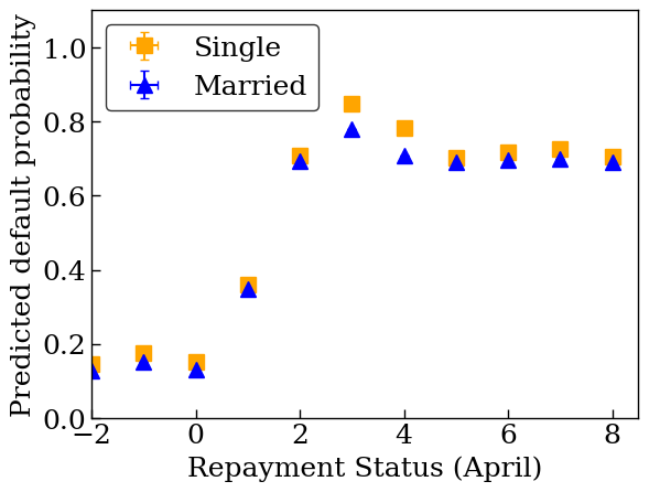
訓練未受限制 (非單調) 的校正晶格模型

model_config = tfl.configs.CalibratedLatticeConfig(
    feature_configs=[
        tfl.configs.FeatureConfig(
            name='MARRIAGE',
            lattice_size=3,
            pwl_calibration_num_keypoints=2,
            monotonicity=0,
            pwl_calibration_always_monotonic=False,
        ),
        tfl.configs.FeatureConfig(
            name='PAY_0',
            lattice_size=3,
            pwl_calibration_num_keypoints=16,
            monotonicity=0,
            pwl_calibration_always_monotonic=False,
        ),
    ],
    output_calibration=True,
    output_initialization=np.linspace(-2, 2, num=8),
)

feature_keypoints = tfl.premade_lib.compute_feature_keypoints(
    feature_configs=model_config.feature_configs,
    features=dfs["credit_train"][['MARRIAGE', 'PAY_0', 'default']],
)
tfl.premade_lib.set_feature_keypoints(
    feature_configs=model_config.feature_configs,
    feature_keypoints=feature_keypoints,
    add_missing_feature_configs=False,
)

nomon_lattice_model = tfl.premade.CalibratedLattice(model_config=model_config)

nomon_lattice_model.compile(
    loss=keras.losses.BinaryCrossentropy(from_logits=True),
    metrics=[
        keras.metrics.BinaryAccuracy(name='accuracy'),
    ],
    optimizer=keras.optimizers.Adam(LEARNING_RATES),
)
nomon_lattice_model.fit(datasets['credit_train'], epochs=NUM_EPOCHS, verbose=0)

train_acc = nomon_lattice_model.evaluate(datasets['credit_train'])[1]
val_acc = nomon_lattice_model.evaluate(datasets['credit_val'])[1]
test_acc = nomon_lattice_model.evaluate(datasets['credit_test'])[1]
print(
    'accuracies for train: %f, val: %f, test: %f'
    % (train_acc, val_acc, test_acc)
)

83/83 [==============================] - 0s 1ms/step - loss: 0.4537 - accuracy: 0.8186
12/12 [==============================] - 0s 2ms/step - loss: 0.4423 - accuracy: 0.8291
24/24 [==============================] - 0s 1ms/step - loss: 0.4547 - accuracy: 0.8168
accuracies for train: 0.818619, val: 0.829085, test: 0.816835

plot_predictions_credit(dfs['credit_train'], nomon_lattice_model, 'PAY_0')

657/657 [==============================] - 1s 1ms/step
/tmpfs/tmp/ipykernel_10210/4037607942.py:3: FutureWarning: The default of observed=False is deprecated and will be changed to True in a future version of pandas. Pass observed=False to retain current behavior or observed=True to adopt the future default and silence this warning.
  data = df[[x_col, y_col]].groupby(xbins).agg(['mean', 'sem'])
/tmpfs/tmp/ipykernel_10210/4037607942.py:3: FutureWarning: The default of observed=False is deprecated and will be changed to True in a future version of pandas. Pass observed=False to retain current behavior or observed=True to adopt the future default and silence this warning.
  data = df[[x_col, y_col]].groupby(xbins).agg(['mean', 'sem'])

訓練單調校正晶格模型

model_config.feature_configs[0].monotonicity = 1
model_config.feature_configs[1].monotonicity = 1

mon_lattice_model = tfl.premade.CalibratedLattice(model_config=model_config)

mon_lattice_model.compile(
    loss=keras.losses.BinaryCrossentropy(from_logits=True),
    metrics=[
        keras.metrics.BinaryAccuracy(name='accuracy'),
    ],
    optimizer=keras.optimizers.Adam(LEARNING_RATES),
)
mon_lattice_model.fit(datasets['credit_train'], epochs=NUM_EPOCHS, verbose=0)

train_acc = mon_lattice_model.evaluate(datasets['credit_train'])[1]
val_acc = mon_lattice_model.evaluate(datasets['credit_val'])[1]
test_acc = mon_lattice_model.evaluate(datasets['credit_test'])[1]
print(
    'accuracies for train: %f, val: %f, test: %f'
    % (train_acc, val_acc, test_acc)
)

83/83 [==============================] - 0s 1ms/step - loss: 0.4548 - accuracy: 0.8188
12/12 [==============================] - 0s 2ms/step - loss: 0.4426 - accuracy: 0.8301
24/24 [==============================] - 0s 1ms/step - loss: 0.4551 - accuracy: 0.8172
accuracies for train: 0.818762, val: 0.830065, test: 0.817172

plot_predictions_credit(dfs['credit_train'], mon_lattice_model, 'PAY_0')

657/657 [==============================] - 1s 1ms/step
/tmpfs/tmp/ipykernel_10210/4037607942.py:3: FutureWarning: The default of observed=False is deprecated and will be changed to True in a future version of pandas. Pass observed=False to retain current behavior or observed=True to adopt the future default and silence this warning.
  data = df[[x_col, y_col]].groupby(xbins).agg(['mean', 'sem'])
/tmpfs/tmp/ipykernel_10210/4037607942.py:3: FutureWarning: The default of observed=False is deprecated and will be changed to True in a future version of pandas. Pass observed=False to retain current behavior or observed=True to adopt the future default and silence this warning.
  data = df[[x_col, y_col]].groupby(xbins).agg(['mean', 'sem'])