
|
|
|
 在 GitHub 上檢視原始碼 在 GitHub 上檢視原始碼
|
|
總覽
預製模型是為一般用途案例快速且輕鬆建構 TFL keras.Model 執行個體的方法。本指南概述建構 TFL 預製模型並訓練/測試模型所需的步驟。
設定
安裝 TF Lattice 套件
pip install --pre -U tensorflow tf-keras tensorflow-lattice pydot graphviz
匯入必要套件
import tensorflow as tf

import copy
import logging
import numpy as np
import pandas as pd
import sys
import tensorflow_lattice as tfl
logging.disable(sys.maxsize)
# Use Keras 2.
version_fn = getattr(tf.keras, "version", None)
if version_fn and version_fn().startswith("3."):
  import tf_keras as keras
else:
  keras = tf.keras
設定本指南中用於訓練的預設值
LEARNING_RATE = 0.01
BATCH_SIZE = 128
NUM_EPOCHS = 500
PREFITTING_NUM_EPOCHS = 10
下載 UCI Statlog (心臟) 資料集
heart_csv_file = keras.utils.get_file(
    'heart.csv',
    'http://storage.googleapis.com/download.tensorflow.org/data/heart.csv')
heart_df = pd.read_csv(heart_csv_file)
thal_vocab_list = ['normal', 'fixed', 'reversible']
heart_df['thal'] = heart_df['thal'].map(
    {v: i for i, v in enumerate(thal_vocab_list)})
heart_df = heart_df.astype(float)

heart_train_size = int(len(heart_df) * 0.8)
heart_train_dict = dict(heart_df[:heart_train_size])
heart_test_dict = dict(heart_df[heart_train_size:])

# This ordering of input features should match the feature configs. If no
# feature config relies explicitly on the data (i.e. all are 'quantiles'),
# then you can construct the feature_names list by simply iterating over each
# feature config and extracting it's name.
feature_names = [
    'age', 'sex', 'cp', 'chol', 'fbs', 'trestbps', 'thalach', 'restecg',
    'exang', 'oldpeak', 'slope', 'ca', 'thal'
]

# Since we have some features that manually construct their input keypoints,
# we need an index mapping of the feature names.
feature_name_indices = {name: index for index, name in enumerate(feature_names)}

label_name = 'target'
heart_train_xs = [
    heart_train_dict[feature_name] for feature_name in feature_names
]
heart_test_xs = [heart_test_dict[feature_name] for feature_name in feature_names]
heart_train_ys = heart_train_dict[label_name]
heart_test_ys = heart_test_dict[label_name]
特徵設定
特徵校正和個別特徵設定是使用 tfl.configs.FeatureConfig 進行設定。特徵設定包括單調性限制、個別特徵正規化 (請參閱 tfl.configs.RegularizerConfig) 以及格狀模型的格狀大小。
請注意,我們必須完整指定任何我們想要模型辨識的特徵的特徵設定。否則,模型將無法得知這類特徵存在。
定義我們的特徵設定
現在我們可以計算分位數,我們為每個想要模型當做輸入的特徵定義特徵設定。
# Features:
# - age
# - sex
# - cp        chest pain type (4 values)
# - trestbps  resting blood pressure
# - chol      serum cholestoral in mg/dl
# - fbs       fasting blood sugar > 120 mg/dl
# - restecg   resting electrocardiographic results (values 0,1,2)
# - thalach   maximum heart rate achieved
# - exang     exercise induced angina
# - oldpeak   ST depression induced by exercise relative to rest
# - slope     the slope of the peak exercise ST segment
# - ca        number of major vessels (0-3) colored by flourosopy
# - thal      normal; fixed defect; reversable defect
#
# Feature configs are used to specify how each feature is calibrated and used.
heart_feature_configs = [
    tfl.configs.FeatureConfig(
        name='age',
        lattice_size=3,
        monotonicity='increasing',
        # We must set the keypoints manually.
        pwl_calibration_num_keypoints=5,
        pwl_calibration_input_keypoints='quantiles',
        pwl_calibration_clip_max=100,
        # Per feature regularization.
        regularizer_configs=[
            tfl.configs.RegularizerConfig(name='calib_wrinkle', l2=0.1),
        ],
    ),
    tfl.configs.FeatureConfig(
        name='sex',
        num_buckets=2,
    ),
    tfl.configs.FeatureConfig(
        name='cp',
        monotonicity='increasing',
        # Keypoints that are uniformly spaced.
        pwl_calibration_num_keypoints=4,
        pwl_calibration_input_keypoints=np.linspace(
            np.min(heart_train_xs[feature_name_indices['cp']]),
            np.max(heart_train_xs[feature_name_indices['cp']]),
            num=4),
    ),
    tfl.configs.FeatureConfig(
        name='chol',
        monotonicity='increasing',
        # Explicit input keypoints initialization.
        pwl_calibration_input_keypoints=[126.0, 210.0, 247.0, 286.0, 564.0],
        # Calibration can be forced to span the full output range by clamping.
        pwl_calibration_clamp_min=True,
        pwl_calibration_clamp_max=True,
        # Per feature regularization.
        regularizer_configs=[
            tfl.configs.RegularizerConfig(name='calib_hessian', l2=1e-4),
        ],
    ),
    tfl.configs.FeatureConfig(
        name='fbs',
        # Partial monotonicity: output(0) <= output(1)
        monotonicity=[(0, 1)],
        num_buckets=2,
    ),
    tfl.configs.FeatureConfig(
        name='trestbps',
        monotonicity='decreasing',
        pwl_calibration_num_keypoints=5,
        pwl_calibration_input_keypoints='quantiles',
    ),
    tfl.configs.FeatureConfig(
        name='thalach',
        monotonicity='decreasing',
        pwl_calibration_num_keypoints=5,
        pwl_calibration_input_keypoints='quantiles',
    ),
    tfl.configs.FeatureConfig(
        name='restecg',
        # Partial monotonicity: output(0) <= output(1), output(0) <= output(2)
        monotonicity=[(0, 1), (0, 2)],
        num_buckets=3,
    ),
    tfl.configs.FeatureConfig(
        name='exang',
        # Partial monotonicity: output(0) <= output(1)
        monotonicity=[(0, 1)],
        num_buckets=2,
    ),
    tfl.configs.FeatureConfig(
        name='oldpeak',
        monotonicity='increasing',
        pwl_calibration_num_keypoints=5,
        pwl_calibration_input_keypoints='quantiles',
    ),
    tfl.configs.FeatureConfig(
        name='slope',
        # Partial monotonicity: output(0) <= output(1), output(1) <= output(2)
        monotonicity=[(0, 1), (1, 2)],
        num_buckets=3,
    ),
    tfl.configs.FeatureConfig(
        name='ca',
        monotonicity='increasing',
        pwl_calibration_num_keypoints=4,
        pwl_calibration_input_keypoints='quantiles',
    ),
    tfl.configs.FeatureConfig(
        name='thal',
        # Partial monotonicity:
        # output(normal) <= output(fixed)
        # output(normal) <= output(reversible)
        monotonicity=[('normal', 'fixed'), ('normal', 'reversible')],
        num_buckets=3,
        # We must specify the vocabulary list in order to later set the
        # monotonicities since we used names and not indices.
        vocabulary_list=thal_vocab_list,
    ),
]
設定單調性和關鍵點
接下來,我們需要確保正確設定我們使用自訂詞彙 (例如上方的 'thal') 的特徵的單調性。
tfl.premade_lib.set_categorical_monotonicities(heart_feature_configs)
最後,我們可以透過計算和設定關鍵點來完成我們的特徵設定。
feature_keypoints = tfl.premade_lib.compute_feature_keypoints(
    feature_configs=heart_feature_configs, features=heart_train_dict)
tfl.premade_lib.set_feature_keypoints(
    feature_configs=heart_feature_configs,
    feature_keypoints=feature_keypoints,
    add_missing_feature_configs=False)
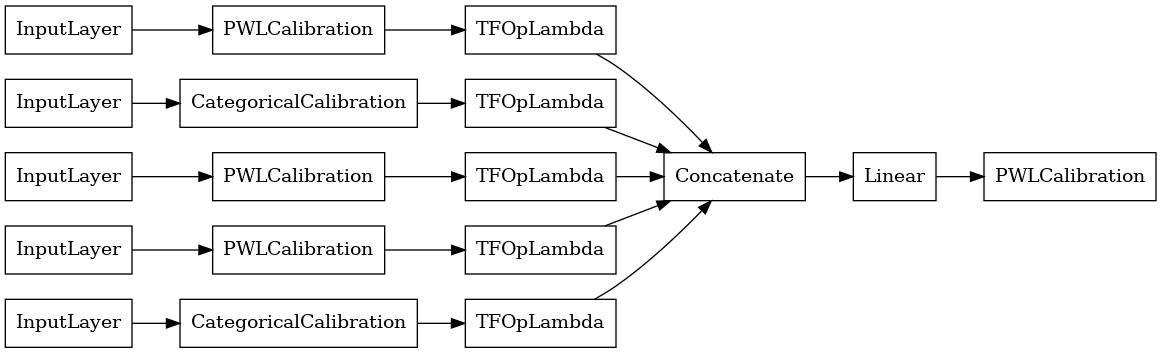
已校正線性模型
若要建構 TFL 預製模型,請先從 tfl.configs 建構模型設定。已校正線性模型是使用 tfl.configs.CalibratedLinearConfig 建構而成。它會在輸入特徵上套用分段線性和類別校正,然後進行線性組合和選用的輸出分段線性校正。當使用輸出校正或指定輸出邊界時,線性層會對已校正輸入套用加權平均。
此範例會在前 5 個特徵上建立已校正線性模型。
# Model config defines the model structure for the premade model.
linear_model_config = tfl.configs.CalibratedLinearConfig(
    feature_configs=heart_feature_configs[:5],
    use_bias=True,
    output_calibration=True,
    output_calibration_num_keypoints=10,
    # We initialize the output to [-2.0, 2.0] since we'll be using logits.
    output_initialization=np.linspace(-2.0, 2.0, num=10),
    regularizer_configs=[
        # Regularizer for the output calibrator.
        tfl.configs.RegularizerConfig(name='output_calib_hessian', l2=1e-4),
    ])
# A CalibratedLinear premade model constructed from the given model config.
linear_model = tfl.premade.CalibratedLinear(linear_model_config)
# Let's plot our model.
keras.utils.plot_model(linear_model, show_layer_names=False, rankdir='LR')
2024-03-23 11:24:50.795913: E external/local_xla/xla/stream_executor/cuda/cuda_driver.cc:282] failed call to cuInit: CUDA_ERROR_NO_DEVICE: no CUDA-capable device is detected
現在,如同任何其他 keras.Model 一樣,我們將模型編譯並調整到我們的資料。
linear_model.compile(
    loss=keras.losses.BinaryCrossentropy(from_logits=True),
    metrics=[keras.metrics.AUC(from_logits=True)],
    optimizer=keras.optimizers.Adam(LEARNING_RATE))
linear_model.fit(
    heart_train_xs[:5],
    heart_train_ys,
    epochs=NUM_EPOCHS,
    batch_size=BATCH_SIZE,
    verbose=False)
<tf_keras.src.callbacks.History at 0x7f2e340ce580>
在訓練我們的模型之後,我們可以在我們的測試集上評估它。
print('Test Set Evaluation...')
print(linear_model.evaluate(heart_test_xs[:5], heart_test_ys))
Test Set Evaluation...
2/2 [==============================] - 1s 7ms/step - loss: 0.4746 - auc: 0.8271
[0.47455987334251404, 0.8270676732063293]
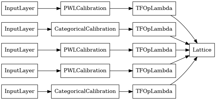
已校正格狀模型
已校正格狀模型是使用 tfl.configs.CalibratedLatticeConfig 建構而成。已校正格狀模型會在輸入特徵上套用分段線性和類別校正,然後是格狀模型和選用的輸出分段線性校正。
此範例會在前 5 個特徵上建立已校正格狀模型。
# This is a calibrated lattice model: inputs are calibrated, then combined
# non-linearly using a lattice layer.
lattice_model_config = tfl.configs.CalibratedLatticeConfig(
    feature_configs=heart_feature_configs[:5],
    # We initialize the output to [-2.0, 2.0] since we'll be using logits.
    output_initialization=[-2.0, 2.0],
    regularizer_configs=[
        # Torsion regularizer applied to the lattice to make it more linear.
        tfl.configs.RegularizerConfig(name='torsion', l2=1e-2),
        # Globally defined calibration regularizer is applied to all features.
        tfl.configs.RegularizerConfig(name='calib_hessian', l2=1e-2),
    ])
# A CalibratedLattice premade model constructed from the given model config.
lattice_model = tfl.premade.CalibratedLattice(lattice_model_config)
# Let's plot our model.
keras.utils.plot_model(lattice_model, show_layer_names=False, rankdir='LR')
如同先前一樣,我們編譯、調整和評估我們的模型。
lattice_model.compile(
    loss=keras.losses.BinaryCrossentropy(from_logits=True),
    metrics=[keras.metrics.AUC(from_logits=True)],
    optimizer=keras.optimizers.Adam(LEARNING_RATE))
lattice_model.fit(
    heart_train_xs[:5],
    heart_train_ys,
    epochs=NUM_EPOCHS,
    batch_size=BATCH_SIZE,
    verbose=False)
print('Test Set Evaluation...')
print(lattice_model.evaluate(heart_test_xs[:5], heart_test_ys))
Test Set Evaluation...
2/2 [==============================] - 1s 8ms/step - loss: 0.4731 - auc_1: 0.8327
[0.47311311960220337, 0.8327068090438843]
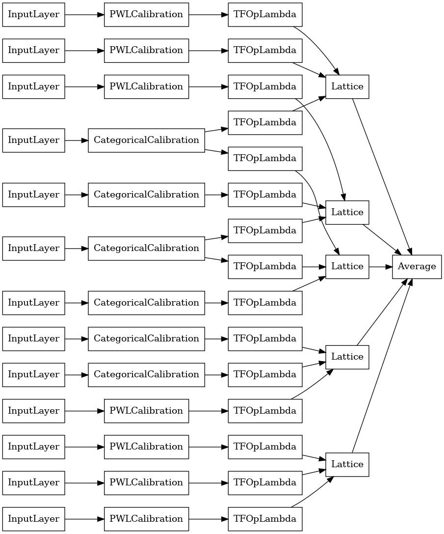
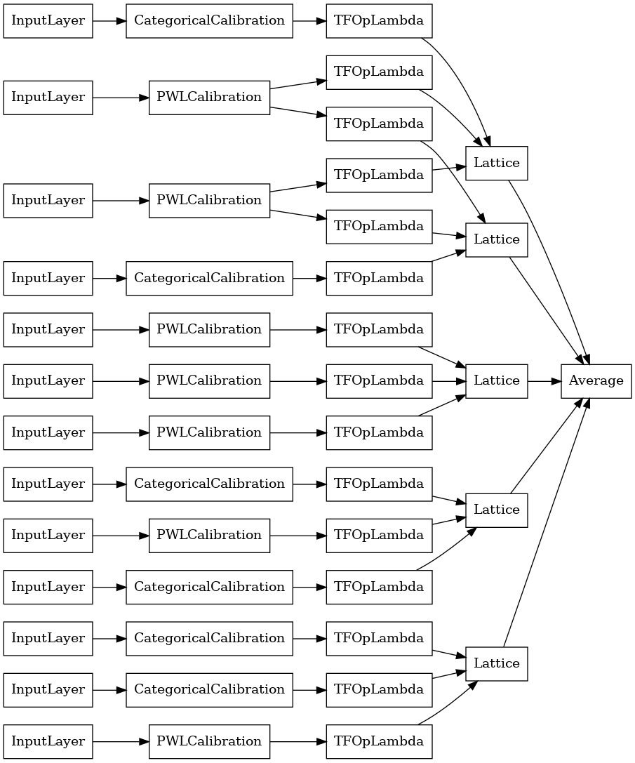
已校正格狀集成模型
當特徵數量很大時,您可以使用集成模型,它會為特徵子集建立多個較小的格狀,並平均其輸出,而不是只建立單一巨型格狀。集成格狀模型是使用 tfl.configs.CalibratedLatticeEnsembleConfig 建構而成。已校正格狀集成模型會在輸入特徵上套用分段線性和類別校正,然後是格狀模型集成和選用的輸出分段線性校正。
明確格狀集成初始化
如果您已經知道您想要饋送到格狀的特徵子集,則您可以使用特徵名稱明確設定格狀。此範例會建立具有 5 個格狀且每個格狀 3 個特徵的已校正格狀集成模型。
# This is a calibrated lattice ensemble model: inputs are calibrated, then
# combined non-linearly and averaged using multiple lattice layers.
explicit_ensemble_model_config = tfl.configs.CalibratedLatticeEnsembleConfig(
    feature_configs=heart_feature_configs,
    lattices=[['trestbps', 'chol', 'ca'], ['fbs', 'restecg', 'thal'],
              ['fbs', 'cp', 'oldpeak'], ['exang', 'slope', 'thalach'],
              ['restecg', 'age', 'sex']],
    num_lattices=5,
    lattice_rank=3,
    # We initialize the output to [-2.0, 2.0] since we'll be using logits.
    output_initialization=[-2.0, 2.0])
# A CalibratedLatticeEnsemble premade model constructed from the given
# model config.
explicit_ensemble_model = tfl.premade.CalibratedLatticeEnsemble(
    explicit_ensemble_model_config)
# Let's plot our model.
keras.utils.plot_model(
    explicit_ensemble_model, show_layer_names=False, rankdir='LR')
如同先前一樣,我們編譯、調整和評估我們的模型。
explicit_ensemble_model.compile(
    loss=keras.losses.BinaryCrossentropy(from_logits=True),
    metrics=[keras.metrics.AUC(from_logits=True)],
    optimizer=keras.optimizers.Adam(LEARNING_RATE))
explicit_ensemble_model.fit(
    heart_train_xs,
    heart_train_ys,
    epochs=NUM_EPOCHS,
    batch_size=BATCH_SIZE,
    verbose=False)
print('Test Set Evaluation...')
print(explicit_ensemble_model.evaluate(heart_test_xs, heart_test_ys))
Test Set Evaluation...
2/2 [==============================] - 1s 9ms/step - loss: 0.3797 - auc_2: 0.8979
[0.37971189618110657, 0.8978697061538696]
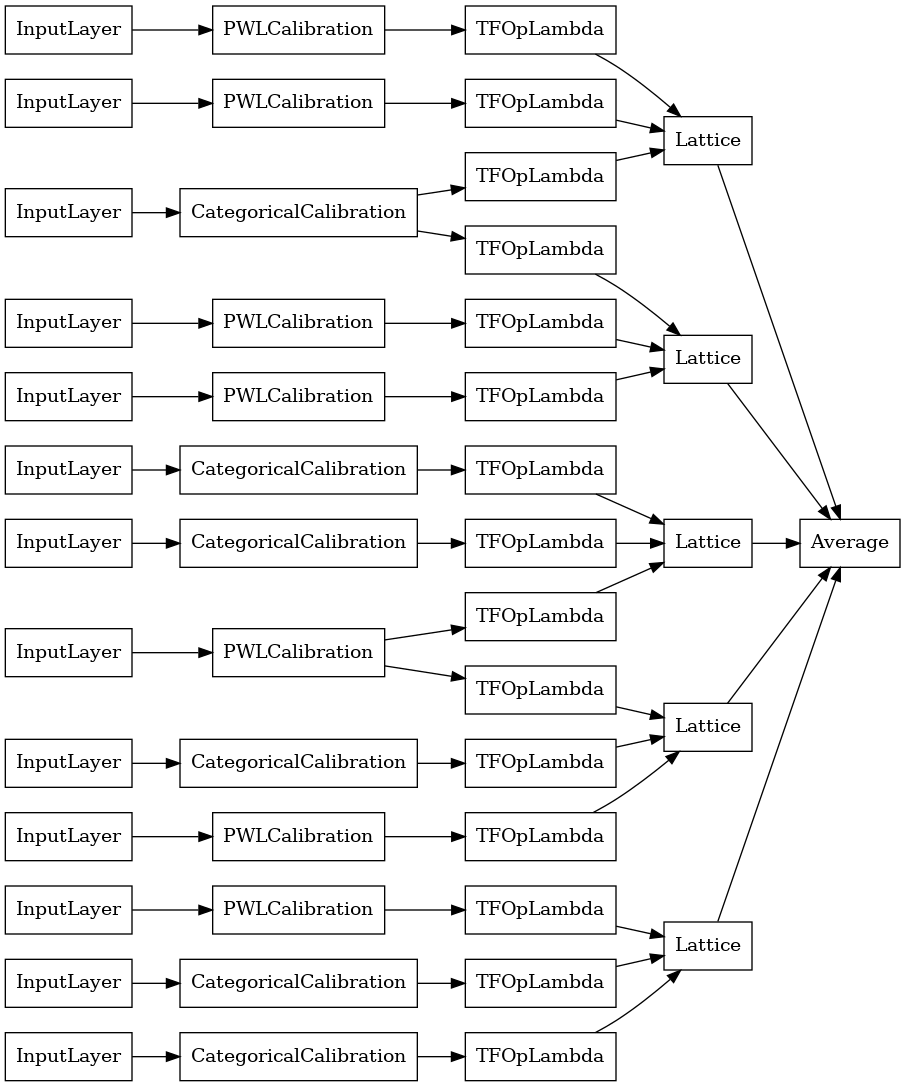
隨機格狀集成
如果您不確定要將哪些特徵子集饋送到您的格狀,另一個選項是為每個格狀使用隨機特徵子集。此範例會建立具有 5 個格狀且每個格狀 3 個特徵的已校正格狀集成模型。
# This is a calibrated lattice ensemble model: inputs are calibrated, then
# combined non-linearly and averaged using multiple lattice layers.
random_ensemble_model_config = tfl.configs.CalibratedLatticeEnsembleConfig(
    feature_configs=heart_feature_configs,
    lattices='random',
    num_lattices=5,
    lattice_rank=3,
    # We initialize the output to [-2.0, 2.0] since we'll be using logits.
    output_initialization=[-2.0, 2.0],
    random_seed=42)
# Now we must set the random lattice structure and construct the model.
tfl.premade_lib.set_random_lattice_ensemble(random_ensemble_model_config)
# A CalibratedLatticeEnsemble premade model constructed from the given
# model config.
random_ensemble_model = tfl.premade.CalibratedLatticeEnsemble(
    random_ensemble_model_config)
# Let's plot our model.
keras.utils.plot_model(
    random_ensemble_model, show_layer_names=False, rankdir='LR')
如同先前一樣,我們編譯、調整和評估我們的模型。
random_ensemble_model.compile(
    loss=keras.losses.BinaryCrossentropy(from_logits=True),
    metrics=[keras.metrics.AUC(from_logits=True)],
    optimizer=keras.optimizers.Adam(LEARNING_RATE))
random_ensemble_model.fit(
    heart_train_xs,
    heart_train_ys,
    epochs=NUM_EPOCHS,
    batch_size=BATCH_SIZE,
    verbose=False)
print('Test Set Evaluation...')
print(random_ensemble_model.evaluate(heart_test_xs, heart_test_ys))
Test Set Evaluation...
2/2 [==============================] - 1s 9ms/step - loss: 0.3708 - auc_3: 0.9054
[0.37078964710235596, 0.9053884744644165]
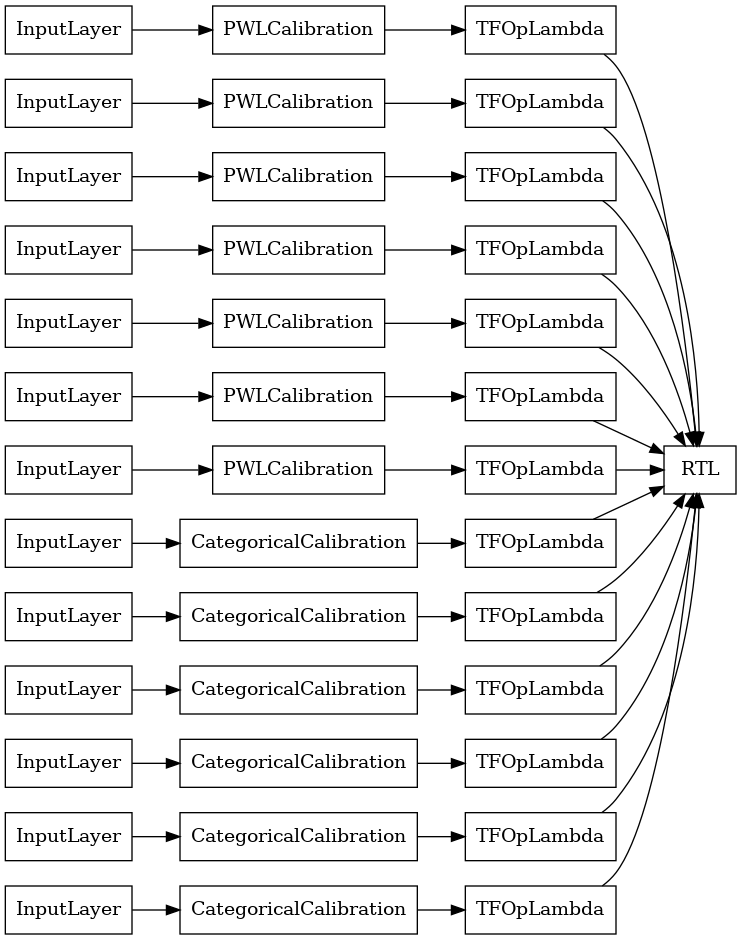
RTL 層隨機格狀集成
當使用隨機格狀集成時,您可以指定模型使用單一 tfl.layers.RTL 層。我們注意到 tfl.layers.RTL 僅支援單調性限制,且所有特徵必須具有相同的格狀大小,且沒有個別特徵正規化。請注意,使用 tfl.layers.RTL 層可讓您擴充到比使用個別 tfl.layers.Lattice 執行個體更大的集成。
此範例會建立具有 5 個格狀且每個格狀 3 個特徵的已校正格狀集成模型。
# Make sure our feature configs have the same lattice size, no per-feature
# regularization, and only monotonicity constraints.
rtl_layer_feature_configs = copy.deepcopy(heart_feature_configs)
for feature_config in rtl_layer_feature_configs:
  feature_config.lattice_size = 2
  feature_config.unimodality = 'none'
  feature_config.reflects_trust_in = None
  feature_config.dominates = None
  feature_config.regularizer_configs = None
# This is a calibrated lattice ensemble model: inputs are calibrated, then
# combined non-linearly and averaged using multiple lattice layers.
rtl_layer_ensemble_model_config = tfl.configs.CalibratedLatticeEnsembleConfig(
    feature_configs=rtl_layer_feature_configs,
    lattices='rtl_layer',
    num_lattices=5,
    lattice_rank=3,
    # We initialize the output to [-2.0, 2.0] since we'll be using logits.
    output_initialization=[-2.0, 2.0],
    random_seed=42)
# A CalibratedLatticeEnsemble premade model constructed from the given
# model config. Note that we do not have to specify the lattices by calling
# a helper function (like before with random) because the RTL Layer will take
# care of that for us.
rtl_layer_ensemble_model = tfl.premade.CalibratedLatticeEnsemble(
    rtl_layer_ensemble_model_config)
# Let's plot our model.
keras.utils.plot_model(
    rtl_layer_ensemble_model, show_layer_names=False, rankdir='LR')
如同先前一樣,我們編譯、調整和評估我們的模型。
rtl_layer_ensemble_model.compile(
    loss=keras.losses.BinaryCrossentropy(from_logits=True),
    metrics=[keras.metrics.AUC(from_logits=True)],
    optimizer=keras.optimizers.Adam(LEARNING_RATE))
rtl_layer_ensemble_model.fit(
    heart_train_xs,
    heart_train_ys,
    epochs=NUM_EPOCHS,
    batch_size=BATCH_SIZE,
    verbose=False)
print('Test Set Evaluation...')
print(rtl_layer_ensemble_model.evaluate(heart_test_xs, heart_test_ys))
Test Set Evaluation...
2/2 [==============================] - 1s 9ms/step - loss: 0.3688 - auc_4: 0.9016
[0.36883750557899475, 0.9016290903091431]
Crystals 格狀集成
Premade 也提供啟發式特徵排列演算法,稱為 Crystals。若要使用 Crystals 演算法,首先我們訓練預先擬合模型,以估計成對特徵互動。然後,我們排列最終集成,以便具有更多非線性互動的特徵位於相同的格狀中。
Premade 程式庫提供輔助函式,用於建構預先擬合模型設定和擷取 Crystals 結構。請注意,預先擬合模型不需要完全訓練,因此幾個週期應該就足夠了。
此範例會建立具有 5 個格狀且每個格狀 3 個特徵的已校正格狀集成模型。
# This is a calibrated lattice ensemble model: inputs are calibrated, then
# combines non-linearly and averaged using multiple lattice layers.
crystals_ensemble_model_config = tfl.configs.CalibratedLatticeEnsembleConfig(
    feature_configs=heart_feature_configs,
    lattices='crystals',
    num_lattices=5,
    lattice_rank=3,
    # We initialize the output to [-2.0, 2.0] since we'll be using logits.
    output_initialization=[-2.0, 2.0],
    random_seed=42)
# Now that we have our model config, we can construct a prefitting model config.
prefitting_model_config = tfl.premade_lib.construct_prefitting_model_config(
    crystals_ensemble_model_config)
# A CalibratedLatticeEnsemble premade model constructed from the given
# prefitting model config.
prefitting_model = tfl.premade.CalibratedLatticeEnsemble(
    prefitting_model_config)
# We can compile and train our prefitting model as we like.
prefitting_model.compile(
    loss=keras.losses.BinaryCrossentropy(from_logits=True),
    optimizer=keras.optimizers.Adam(LEARNING_RATE))
prefitting_model.fit(
    heart_train_xs,
    heart_train_ys,
    epochs=PREFITTING_NUM_EPOCHS,
    batch_size=BATCH_SIZE,
    verbose=False)
# Now that we have our trained prefitting model, we can extract the crystals.
tfl.premade_lib.set_crystals_lattice_ensemble(crystals_ensemble_model_config,
                                              prefitting_model_config,
                                              prefitting_model)
# A CalibratedLatticeEnsemble premade model constructed from the given
# model config.
crystals_ensemble_model = tfl.premade.CalibratedLatticeEnsemble(
    crystals_ensemble_model_config)
# Let's plot our model.
keras.utils.plot_model(
    crystals_ensemble_model, show_layer_names=False, rankdir='LR')
如同先前一樣,我們編譯、調整和評估我們的模型。
crystals_ensemble_model.compile(
    loss=keras.losses.BinaryCrossentropy(from_logits=True),
    metrics=[keras.metrics.AUC(from_logits=True)],
    optimizer=keras.optimizers.Adam(LEARNING_RATE))
crystals_ensemble_model.fit(
    heart_train_xs,
    heart_train_ys,
    epochs=NUM_EPOCHS,
    batch_size=BATCH_SIZE,
    verbose=False)
print('Test Set Evaluation...')
print(crystals_ensemble_model.evaluate(heart_test_xs, heart_test_ys))
Test Set Evaluation...
2/2 [==============================] - 1s 9ms/step - loss: 0.3779 - auc_5: 0.8941
[0.37785840034484863, 0.8941103219985962]