
|
|
|
 在 GitHub 上檢視原始碼 在 GitHub 上檢視原始碼
|
|
在功能化教學課程中,我們將多個功能納入模型,但模型僅由嵌入層組成。我們可以為模型新增更多密集層,以提高其表現力。
一般而言,更深層的模型比更淺層的模型更能學習複雜的模式。例如,我們的使用者模型納入使用者 ID 和時間戳記,以模擬使用者在特定時間點的偏好。淺層模型 (例如,單一嵌入層) 可能只能學習這些功能與電影之間最簡單的關係:特定電影在其發行時最受歡迎,而特定使用者通常偏好恐怖片勝過喜劇片。若要捕捉更複雜的關係 (例如使用者偏好隨時間演變),我們可能需要更深層的模型,其中包含多個堆疊的密集層。
當然,複雜模型也有其缺點。第一個是運算成本,因為較大的模型需要更多記憶體和更多運算才能擬合和服務。第二個是需要更多資料:一般而言,需要更多訓練資料才能充分利用更深層的模型。隨著參數增加,深度模型可能會過度擬合,甚至只是記住訓練範例,而不是學習可以泛化的函數。最後,訓練更深層的模型可能更困難,而且在選擇正規化和學習率等設定時需要更加謹慎。
為真實世界的推薦系統尋找良好的架構是一門複雜的藝術,需要良好的直覺和仔細的超參數調整。例如,模型的深度和寬度、啟動函數、學習率和最佳化工具等因素可能會徹底改變模型的效能。模型選擇的複雜性進一步增加,因為良好的離線評估指標可能與良好的線上效能不符,而且最佳化目標的選擇通常比模型本身的選擇更為關鍵。
儘管如此,投入精力建構和微調較大型模型通常會有所回報。在本教學課程中,我們將說明如何使用 TensorFlow Recommenders 建構深度檢索模型。我們將透過建構漸進複雜的模型來說明這一點,以瞭解這對模型效能有何影響。
初步準備
首先,我們匯入必要的套件。
pip install -q tensorflow-recommenderspip install -q --upgrade tensorflow-datasets
import os
import tempfile

%matplotlib inline
import matplotlib.pyplot as plt

import numpy as np
import tensorflow as tf
import tensorflow_datasets as tfds

import tensorflow_recommenders as tfrs

plt.style.use('seaborn-whitegrid')
2022-12-14 13:06:15.089641: W tensorflow/compiler/xla/stream_executor/platform/default/dso_loader.cc:64] Could not load dynamic library 'libnvinfer.so.7'; dlerror: libnvinfer.so.7: cannot open shared object file: No such file or directory
2022-12-14 13:06:15.089741: W tensorflow/compiler/xla/stream_executor/platform/default/dso_loader.cc:64] Could not load dynamic library 'libnvinfer_plugin.so.7'; dlerror: libnvinfer_plugin.so.7: cannot open shared object file: No such file or directory
2022-12-14 13:06:15.089751: W tensorflow/compiler/tf2tensorrt/utils/py_utils.cc:38] TF-TRT Warning: Cannot dlopen some TensorRT libraries. If you would like to use Nvidia GPU with TensorRT, please make sure the missing libraries mentioned above are installed properly.
/tmpfs/tmp/ipykernel_91398/2468769046.py:13: MatplotlibDeprecationWarning: The seaborn styles shipped by Matplotlib are deprecated since 3.6, as they no longer correspond to the styles shipped by seaborn. However, they will remain available as 'seaborn-v0_8-<style>'. Alternatively, directly use the seaborn API instead.
  plt.style.use('seaborn-whitegrid')
在本教學課程中,我們將使用功能化教學課程中的模型來產生嵌入。因此,我們只會使用使用者 ID、時間戳記和電影標題功能。
ratings = tfds.load("movielens/100k-ratings", split="train")
movies = tfds.load("movielens/100k-movies", split="train")

ratings = ratings.map(lambda x: {
    "movie_title": x["movie_title"],
    "user_id": x["user_id"],
    "timestamp": x["timestamp"],
})
movies = movies.map(lambda x: x["movie_title"])
WARNING:tensorflow:From /tmpfs/src/tf_docs_env/lib/python3.9/site-packages/tensorflow/python/autograph/pyct/static_analysis/liveness.py:83: Analyzer.lamba_check (from tensorflow.python.autograph.pyct.static_analysis.liveness) is deprecated and will be removed after 2023-09-23.
Instructions for updating:
Lambda fuctions will be no more assumed to be used in the statement where they are used, or at least in the same block. https://github.com/tensorflow/tensorflow/issues/56089
我們也會執行一些內務處理,以準備功能詞彙表。
timestamps = np.concatenate(list(ratings.map(lambda x: x["timestamp"]).batch(100)))

max_timestamp = timestamps.max()
min_timestamp = timestamps.min()

timestamp_buckets = np.linspace(
    min_timestamp, max_timestamp, num=1000,
)

unique_movie_titles = np.unique(np.concatenate(list(movies.batch(1000))))
unique_user_ids = np.unique(np.concatenate(list(ratings.batch(1_000).map(
    lambda x: x["user_id"]))))
模型定義
查詢模型
我們從功能化教學課程中定義的使用者模型開始,作為我們模型的第一層,負責將原始輸入範例轉換為功能嵌入。
class UserModel(tf.keras.Model):

  def __init__(self):
    super().__init__()

    self.user_embedding = tf.keras.Sequential([
        tf.keras.layers.StringLookup(
            vocabulary=unique_user_ids, mask_token=None),
        tf.keras.layers.Embedding(len(unique_user_ids) + 1, 32),
    ])
    self.timestamp_embedding = tf.keras.Sequential([
        tf.keras.layers.Discretization(timestamp_buckets.tolist()),
        tf.keras.layers.Embedding(len(timestamp_buckets) + 1, 32),
    ])
    self.normalized_timestamp = tf.keras.layers.Normalization(
        axis=None
    )

    self.normalized_timestamp.adapt(timestamps)

  def call(self, inputs):
    # Take the input dictionary, pass it through each input layer,
    # and concatenate the result.
    return tf.concat([
        self.user_embedding(inputs["user_id"]),
        self.timestamp_embedding(inputs["timestamp"]),
        tf.reshape(self.normalized_timestamp(inputs["timestamp"]), (-1, 1)),
    ], axis=1)
定義更深層的模型需要我們在此第一個輸入之上堆疊模式層。逐漸變窄的層堆疊 (以啟動函數分隔) 是一種常見模式
                            +----------------------+
                            |      128 x 64        |
                            +----------------------+
                                       | relu
                          +--------------------------+
                          |        256 x 128         |
                          +--------------------------+
                                       | relu
                        +------------------------------+
                        |          ... x 256           |
                        +------------------------------+
由於深度線性模型的表現力不比淺層線性模型強,因此我們對最後一個隱藏層以外的所有層都使用 ReLU 啟動。最後一個隱藏層不使用任何啟動函數:使用啟動函數會限制最終嵌入的輸出空間,並可能對模型效能產生負面影響。例如,如果在投影層中使用 ReLU,則輸出嵌入中的所有元件都會是非負數。
我們將在這裡嘗試類似的方法。為了方便實驗不同的深度,讓我們定義一個模型,其深度 (和寬度) 由一組建構函式參數定義。
class QueryModel(tf.keras.Model):
  """Model for encoding user queries."""

  def __init__(self, layer_sizes):
    """Model for encoding user queries.

    Args:
      layer_sizes:
        A list of integers where the i-th entry represents the number of units
        the i-th layer contains.
    """
    super().__init__()

    # We first use the user model for generating embeddings.
    self.embedding_model = UserModel()

    # Then construct the layers.
    self.dense_layers = tf.keras.Sequential()

    # Use the ReLU activation for all but the last layer.
    for layer_size in layer_sizes[:-1]:
      self.dense_layers.add(tf.keras.layers.Dense(layer_size, activation="relu"))

    # No activation for the last layer.
    for layer_size in layer_sizes[-1:]:
      self.dense_layers.add(tf.keras.layers.Dense(layer_size))

  def call(self, inputs):
    feature_embedding = self.embedding_model(inputs)
    return self.dense_layers(feature_embedding)
layer_sizes 參數提供模型的深度和寬度。我們可以變更它來實驗更淺層或更深層的模型。
候選模型
我們可以對電影模型採用相同的方法。同樣地,我們從功能化教學課程中的 MovieModel 開始
class MovieModel(tf.keras.Model):

  def __init__(self):
    super().__init__()

    max_tokens = 10_000

    self.title_embedding = tf.keras.Sequential([
      tf.keras.layers.StringLookup(
          vocabulary=unique_movie_titles,mask_token=None),
      tf.keras.layers.Embedding(len(unique_movie_titles) + 1, 32)
    ])

    self.title_vectorizer = tf.keras.layers.TextVectorization(
        max_tokens=max_tokens)

    self.title_text_embedding = tf.keras.Sequential([
      self.title_vectorizer,
      tf.keras.layers.Embedding(max_tokens, 32, mask_zero=True),
      tf.keras.layers.GlobalAveragePooling1D(),
    ])

    self.title_vectorizer.adapt(movies)

  def call(self, titles):
    return tf.concat([
        self.title_embedding(titles),
        self.title_text_embedding(titles),
    ], axis=1)
並使用隱藏層擴充它
class CandidateModel(tf.keras.Model):
  """Model for encoding movies."""

  def __init__(self, layer_sizes):
    """Model for encoding movies.

    Args:
      layer_sizes:
        A list of integers where the i-th entry represents the number of units
        the i-th layer contains.
    """
    super().__init__()

    self.embedding_model = MovieModel()

    # Then construct the layers.
    self.dense_layers = tf.keras.Sequential()

    # Use the ReLU activation for all but the last layer.
    for layer_size in layer_sizes[:-1]:
      self.dense_layers.add(tf.keras.layers.Dense(layer_size, activation="relu"))

    # No activation for the last layer.
    for layer_size in layer_sizes[-1:]:
      self.dense_layers.add(tf.keras.layers.Dense(layer_size))

  def call(self, inputs):
    feature_embedding = self.embedding_model(inputs)
    return self.dense_layers(feature_embedding)
組合模型
定義 QueryModel 和 CandidateModel 後,我們可以將組合模型放在一起,並實作我們的損失和指標邏輯。為了簡化操作,我們將強制查詢模型和候選模型的模型結構相同。
class MovielensModel(tfrs.models.Model):

  def __init__(self, layer_sizes):
    super().__init__()
    self.query_model = QueryModel(layer_sizes)
    self.candidate_model = CandidateModel(layer_sizes)
    self.task = tfrs.tasks.Retrieval(
        metrics=tfrs.metrics.FactorizedTopK(
            candidates=movies.batch(128).map(self.candidate_model),
        ),
    )

  def compute_loss(self, features, training=False):
    # We only pass the user id and timestamp features into the query model. This
    # is to ensure that the training inputs would have the same keys as the
    # query inputs. Otherwise the discrepancy in input structure would cause an
    # error when loading the query model after saving it.
    query_embeddings = self.query_model({
        "user_id": features["user_id"],
        "timestamp": features["timestamp"],
    })
    movie_embeddings = self.candidate_model(features["movie_title"])

    return self.task(
        query_embeddings, movie_embeddings, compute_metrics=not training)
訓練模型
準備資料
首先,我們將資料分割成訓練集和測試集。
tf.random.set_seed(42)
shuffled = ratings.shuffle(100_000, seed=42, reshuffle_each_iteration=False)

train = shuffled.take(80_000)
test = shuffled.skip(80_000).take(20_000)

cached_train = train.shuffle(100_000).batch(2048)
cached_test = test.batch(4096).cache()
淺層模型
我們已準備好試用我們的第一個淺層模型!
num_epochs = 300

model = MovielensModel([32])
model.compile(optimizer=tf.keras.optimizers.Adagrad(0.1))

one_layer_history = model.fit(
    cached_train,
    validation_data=cached_test,
    validation_freq=5,
    epochs=num_epochs,
    verbose=0)

accuracy = one_layer_history.history["val_factorized_top_k/top_100_categorical_accuracy"][-1]
print(f"Top-100 accuracy: {accuracy:.2f}.")
Top-100 accuracy: 0.27.
這為我們提供了約 0.27 的前 100 項準確度。我們可以將此作為評估更深層模型的參考點。
更深層的模型
那麼具有兩層的更深層模型呢?
model = MovielensModel([64, 32])
model.compile(optimizer=tf.keras.optimizers.Adagrad(0.1))

two_layer_history = model.fit(
    cached_train,
    validation_data=cached_test,
    validation_freq=5,
    epochs=num_epochs,
    verbose=0)

accuracy = two_layer_history.history["val_factorized_top_k/top_100_categorical_accuracy"][-1]
print(f"Top-100 accuracy: {accuracy:.2f}.")
Top-100 accuracy: 0.28.
此處的準確度為 0.29,比淺層模型好很多。
我們可以繪製驗證準確度曲線來說明這一點
num_validation_runs = len(one_layer_history.history["val_factorized_top_k/top_100_categorical_accuracy"])
epochs = [(x + 1)* 5 for x in range(num_validation_runs)]

plt.plot(epochs, one_layer_history.history["val_factorized_top_k/top_100_categorical_accuracy"], label="1 layer")
plt.plot(epochs, two_layer_history.history["val_factorized_top_k/top_100_categorical_accuracy"], label="2 layers")
plt.title("Accuracy vs epoch")
plt.xlabel("epoch")
plt.ylabel("Top-100 accuracy");
plt.legend()
<matplotlib.legend.Legend at 0x7f5d9402a670>
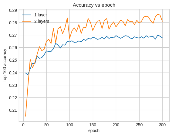
即使在訓練的早期,較大的模型也明顯且穩定地領先於淺層模型,這表示新增深度有助於模型捕捉資料中更細微的關係。
但是,即使是更深層的模型也不一定更好。以下模型將深度擴充到三層
model = MovielensModel([128, 64, 32])
model.compile(optimizer=tf.keras.optimizers.Adagrad(0.1))

three_layer_history = model.fit(
    cached_train,
    validation_data=cached_test,
    validation_freq=5,
    epochs=num_epochs,
    verbose=0)

accuracy = three_layer_history.history["val_factorized_top_k/top_100_categorical_accuracy"][-1]
print(f"Top-100 accuracy: {accuracy:.2f}.")
Top-100 accuracy: 0.25.
事實上,我們沒有看到比淺層模型更好的改進
plt.plot(epochs, one_layer_history.history["val_factorized_top_k/top_100_categorical_accuracy"], label="1 layer")
plt.plot(epochs, two_layer_history.history["val_factorized_top_k/top_100_categorical_accuracy"], label="2 layers")
plt.plot(epochs, three_layer_history.history["val_factorized_top_k/top_100_categorical_accuracy"], label="3 layers")
plt.title("Accuracy vs epoch")
plt.xlabel("epoch")
plt.ylabel("Top-100 accuracy");
plt.legend()
<matplotlib.legend.Legend at 0x7f5d9406d070>
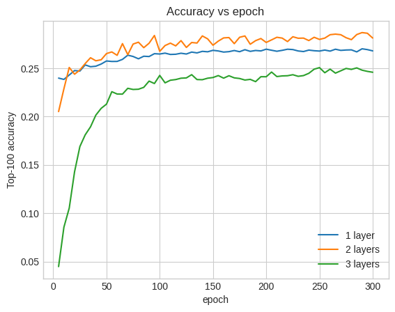
這很好地說明了以下事實:更深層和更大的模型雖然能夠提供卓越的效能,但通常需要非常仔細的微調。例如,在本教學課程中,我們使用了單一的固定學習率。其他選擇可能會產生非常不同的結果,值得探索。
透過適當的微調和足夠的資料,在許多情況下,投入精力建構更大和更深層的模型是值得的:更大的模型可以大幅提高預測準確度。
後續步驟
在本教學課程中,我們使用密集層和啟動函數擴充了檢索模型。若要瞭解如何建立不僅可以執行檢索工作,還可以執行評分工作的模型,請參閱多工教學課程。