
|
|
|
 在 GitHub 上檢視原始碼 在 GitHub 上檢視原始碼
|
|
本教學課程示範如何使用深度與交叉網路 (DCN) 有效地學習特徵交叉。
背景
什麼是特徵交叉?為什麼它們很重要? 想像一下,我們正在建構一個推薦系統,向顧客銷售果汁機。那麼,顧客過去的購買歷史記錄,例如 purchased_bananas 和 purchased_cooking_books,或地理特徵,都是單一特徵。如果有人同時購買了香蕉和食譜,那麼這位顧客更有可能點擊推薦的果汁機。purchased_bananas 和 purchased_cooking_books 的組合稱為特徵交叉,它提供了超出個別特徵的額外互動資訊。
學習特徵交叉的挑戰是什麼? 在 Web 規模的應用程式中,資料大多是類別型的,導致龐大且稀疏的特徵空間。在這種情況下識別有效的特徵交叉通常需要手動特徵工程或詳盡的搜尋。傳統的前饋多層感知器 (MLP) 模型是通用函數逼近器;但是,它們甚至無法有效逼近二階或三階特徵交叉 [1, 2]。
什麼是深度與交叉網路 (DCN)? DCN 旨在更有效地學習顯式和有界度的交叉特徵。它從輸入層(通常是嵌入層)開始,接著是一個交叉網路,其中包含多個交叉層,用於模擬顯式特徵互動,然後與一個深度網路結合,用於模擬隱式特徵互動。
- 交叉網路。這是 DCN 的核心。它在每一層顯式應用特徵交叉,最高多項式次數隨著層深度增加。下圖顯示了第 \((i+1)\) 個交叉層。
- 深度網路。它是傳統的前饋多層感知器 (MLP)。
深度網路和交叉網路隨後結合形成 DCN [1]。通常,我們可以將深度網路堆疊在交叉網路之上(堆疊結構);我們也可以將它們並排放置(並行結構)。
在接下來的內容中,我們將首先透過一個玩具範例展示 DCN 的優勢,然後我們將引導您瞭解使用 MovieLen-1M 資料集來利用 DCN 的一些常見方法。
讓我們先安裝和匯入此 Colab 的必要套件。
pip install -q tensorflow-recommenderspip install -q --upgrade tensorflow-datasets
import pprint

%matplotlib inline
import matplotlib.pyplot as plt
from mpl_toolkits.axes_grid1 import make_axes_locatable

import numpy as np
import tensorflow as tf
import tensorflow_datasets as tfds

import tensorflow_recommenders as tfrs
2022-12-14 12:19:17.483745: W tensorflow/compiler/xla/stream_executor/platform/default/dso_loader.cc:64] Could not load dynamic library 'libnvinfer.so.7'; dlerror: libnvinfer.so.7: cannot open shared object file: No such file or directory
2022-12-14 12:19:17.483841: W tensorflow/compiler/xla/stream_executor/platform/default/dso_loader.cc:64] Could not load dynamic library 'libnvinfer_plugin.so.7'; dlerror: libnvinfer_plugin.so.7: cannot open shared object file: No such file or directory
2022-12-14 12:19:17.483851: W tensorflow/compiler/tf2tensorrt/utils/py_utils.cc:38] TF-TRT Warning: Cannot dlopen some TensorRT libraries. If you would like to use Nvidia GPU with TensorRT, please make sure the missing libraries mentioned above are installed properly.
玩具範例
為了說明 DCN 的優點,讓我們透過一個簡單的範例。假設我們有一個資料集,我們試圖模擬顧客點擊果汁機廣告的可能性,其特徵和標籤描述如下。
| 特徵 / 標籤 | 描述 | 值類型 / 範圍 |
|---|---|---|
| \(x_1\) = 國家/地區 | 顧客居住的國家/地區 | 介於 [0, 199] 的整數 |
| \(x_2\) = 香蕉 | 顧客購買的香蕉數量 | 介於 [0, 23] 的整數 |
| \(x_3\) = 食譜 | 顧客購買的食譜數量 | 介於 [0, 5] 的整數 |
| \(y\) | 點擊果汁機廣告的可能性 | -- |
然後,我們讓資料遵循以下底層分佈
\[y = f(x_1, x_2, x_3) = 0.1x_1 + 0.4x_2+0.7x_3 + 0.1x_1x_2+3.1x_2x_3+0.1x_3^2\]
其中可能性 \(y\) 線性地取決於特徵 \(x_i\) 以及 \(x_i\) 之間的乘法互動。在我們的例子中,我們會說購買果汁機 (\(y\)) 的可能性不僅取決於購買香蕉 (\(x_2\)) 或食譜 (\(x_3\)),還取決於一起購買香蕉和食譜 (\(x_2x_3\))。
我們可以按如下方式產生此資料的資料
合成資料產生
我們首先定義如上所述的 \(f(x_1, x_2, x_3)\)。
def get_mixer_data(data_size=100_000, random_seed=42):
  # We need to fix the random seed
  # to make colab runs repeatable.
  rng = np.random.RandomState(random_seed)
  country = rng.randint(200, size=[data_size, 1]) / 200.
  bananas = rng.randint(24, size=[data_size, 1]) / 24.
  cookbooks = rng.randint(6, size=[data_size, 1]) / 6.

  x = np.concatenate([country, bananas, cookbooks], axis=1)

  # # Create 1st-order terms.
  y = 0.1 * country + 0.4 * bananas + 0.7 * cookbooks

  # Create 2nd-order cross terms.
  y += 0.1 * country * bananas + 3.1 * bananas * cookbooks + (
        0.1 * cookbooks * cookbooks)

  return x, y
讓我們產生遵循分佈的資料,並將資料分成 90% 用於訓練,10% 用於測試。
x, y = get_mixer_data()
num_train = 90000
train_x = x[:num_train]
train_y = y[:num_train]
eval_x = x[num_train:]
eval_y = y[num_train:]
模型建構
我們將嘗試交叉網路和深度網路,以說明交叉網路可以為推薦器帶來的優勢。由於我們剛剛建立的資料僅包含二階特徵互動,因此使用單層交叉網路進行說明就足夠了。如果我們想要模擬更高階的特徵互動,我們可以堆疊多個交叉層並使用多層交叉網路。我們將建構的兩個模型是
- 僅具有一個交叉層的交叉網路;
- 具有更寬更深 ReLU 層的深度網路。
我們首先建構一個統一的模型類別,其損失是均方誤差。
class Model(tfrs.Model):

  def __init__(self, model):
    super().__init__()
    self._model = model
    self._logit_layer = tf.keras.layers.Dense(1)

    self.task = tfrs.tasks.Ranking(
      loss=tf.keras.losses.MeanSquaredError(),
      metrics=[
        tf.keras.metrics.RootMeanSquaredError("RMSE")
      ]
    )

  def call(self, x):
    x = self._model(x)
    return self._logit_layer(x)

  def compute_loss(self, features, training=False):
    x, labels = features
    scores = self(x)

    return self.task(
        labels=labels,
        predictions=scores,
    )
然後,我們指定交叉網路(具有 1 個大小為 3 的交叉層)和基於 ReLU 的 DNN(層大小為 [512, 256, 128])
crossnet = Model(tfrs.layers.dcn.Cross())
deepnet = Model(
    tf.keras.Sequential([
      tf.keras.layers.Dense(512, activation="relu"),
      tf.keras.layers.Dense(256, activation="relu"),
      tf.keras.layers.Dense(128, activation="relu")
    ])
)
模型訓練
現在我們已經準備好資料和模型,我們將訓練模型。我們先對資料進行洗牌和批次處理,為模型訓練做準備。
train_data = tf.data.Dataset.from_tensor_slices((train_x, train_y)).batch(1000)
eval_data = tf.data.Dataset.from_tensor_slices((eval_x, eval_y)).batch(1000)
然後,我們定義 epoch 數以及學習率。
epochs = 100
learning_rate = 0.4
好了,一切都準備就緒,讓我們編譯和訓練模型。如果您想查看模型進度,可以將 verbose=True 設定為 True。
crossnet.compile(optimizer=tf.keras.optimizers.Adagrad(learning_rate))
crossnet.fit(train_data, epochs=epochs, verbose=False)
<keras.callbacks.History at 0x7fc688388bb0>
deepnet.compile(optimizer=tf.keras.optimizers.Adagrad(learning_rate))
deepnet.fit(train_data, epochs=epochs, verbose=False)
<keras.callbacks.History at 0x7fc5f0386af0>
模型評估
我們驗證模型在評估資料集上的效能,並報告均方根誤差 (RMSE,越低越好)。
crossnet_result = crossnet.evaluate(eval_data, return_dict=True, verbose=False)
print(f"CrossNet(1 layer) RMSE is {crossnet_result['RMSE']:.4f} "
      f"using {crossnet.count_params()} parameters.")

deepnet_result = deepnet.evaluate(eval_data, return_dict=True, verbose=False)
print(f"DeepNet(large) RMSE is {deepnet_result['RMSE']:.4f} "
      f"using {deepnet.count_params()} parameters.")
CrossNet(1 layer) RMSE is 0.0001 using 16 parameters.
DeepNet(large) RMSE is 0.0933 using 166401 parameters.
我們看到交叉網路實現了比基於 ReLU 的 DNN 低數個數量級的 RMSE,並且參數少了數個數量級。這表明了交叉網路在學習特徵交叉方面的效率。
模型理解
我們已經知道哪些特徵交叉在我們的資料中很重要,檢查我們的模型是否確實學習了重要的特徵交叉會很有趣。這可以透過視覺化 DCN 中學習到的權重矩陣來完成。權重 \(W_{ij}\) 代表學習到的特徵 \(x_i\) 和 \(x_j\) 之間互動的重要性。
mat = crossnet._model._dense.kernel
features = ["country", "purchased_bananas", "purchased_cookbooks"]

plt.figure(figsize=(9,9))
im = plt.matshow(np.abs(mat.numpy()), cmap=plt.cm.Blues)
ax = plt.gca()
divider = make_axes_locatable(plt.gca())
cax = divider.append_axes("right", size="5%", pad=0.05)
plt.colorbar(im, cax=cax)
cax.tick_params(labelsize=10)
_ = ax.set_xticklabels([''] + features, rotation=45, fontsize=10)
_ = ax.set_yticklabels([''] + features, fontsize=10)
/tmpfs/tmp/ipykernel_40470/2879280353.py:11: UserWarning: FixedFormatter should only be used together with FixedLocator
  _ = ax.set_xticklabels([''] + features, rotation=45, fontsize=10)
/tmpfs/tmp/ipykernel_40470/2879280353.py:12: UserWarning: FixedFormatter should only be used together with FixedLocator
  _ = ax.set_yticklabels([''] + features, fontsize=10)
<Figure size 900x900 with 0 Axes>
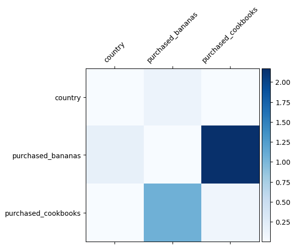
較深的顏色代表更強的學習到的互動 - 在這種情況下,很明顯模型學習到一起購買香蕉和食譜很重要。
如果您有興趣嘗試更複雜的合成資料,請隨時查看 這篇論文。
Movielens 1M 範例
我們現在檢視 DCN 在真實世界資料集上的有效性:Movielens 1M [3]。Movielens 1M 是推薦研究的熱門資料集。它根據使用者相關特徵和電影相關特徵預測使用者的電影評分。我們使用此資料集來示範一些利用 DCN 的常見方法。
資料處理
資料處理程序遵循與基本排名教學課程類似的程序。
ratings = tfds.load("movie_lens/100k-ratings", split="train")
ratings = ratings.map(lambda x: {
    "movie_id": x["movie_id"],
    "user_id": x["user_id"],
    "user_rating": x["user_rating"],
    "user_gender": int(x["user_gender"]),
    "user_zip_code": x["user_zip_code"],
    "user_occupation_text": x["user_occupation_text"],
    "bucketized_user_age": int(x["bucketized_user_age"]),
})
WARNING:absl:The handle "movie_lens" for the MovieLens dataset is deprecated. Prefer using "movielens" instead.
WARNING:tensorflow:From /tmpfs/src/tf_docs_env/lib/python3.9/site-packages/tensorflow/python/autograph/pyct/static_analysis/liveness.py:83: Analyzer.lamba_check (from tensorflow.python.autograph.pyct.static_analysis.liveness) is deprecated and will be removed after 2023-09-23.
Instructions for updating:
Lambda fuctions will be no more assumed to be used in the statement where they are used, or at least in the same block. https://github.com/tensorflow/tensorflow/issues/56089
接下來,我們將資料隨機分成 80% 用於訓練,20% 用於測試。
tf.random.set_seed(42)
shuffled = ratings.shuffle(100_000, seed=42, reshuffle_each_iteration=False)

train = shuffled.take(80_000)
test = shuffled.skip(80_000).take(20_000)
然後,我們為每個特徵建立詞彙表。
feature_names = ["movie_id", "user_id", "user_gender", "user_zip_code",
                 "user_occupation_text", "bucketized_user_age"]

vocabularies = {}

for feature_name in feature_names:
  vocab = ratings.batch(1_000_000).map(lambda x: x[feature_name])
  vocabularies[feature_name] = np.unique(np.concatenate(list(vocab)))
模型建構
我們將建構的模型架構從嵌入層開始,該嵌入層饋送到交叉網路,然後是深度網路。所有特徵的嵌入維度都設定為 32。您也可以為不同的特徵使用不同的嵌入大小。
class DCN(tfrs.Model):

  def __init__(self, use_cross_layer, deep_layer_sizes, projection_dim=None):
    super().__init__()

    self.embedding_dimension = 32

    str_features = ["movie_id", "user_id", "user_zip_code",
                    "user_occupation_text"]
    int_features = ["user_gender", "bucketized_user_age"]

    self._all_features = str_features + int_features
    self._embeddings = {}

    # Compute embeddings for string features.
    for feature_name in str_features:
      vocabulary = vocabularies[feature_name]
      self._embeddings[feature_name] = tf.keras.Sequential(
          [tf.keras.layers.StringLookup(
              vocabulary=vocabulary, mask_token=None),
           tf.keras.layers.Embedding(len(vocabulary) + 1,
                                     self.embedding_dimension)
    ])

    # Compute embeddings for int features.
    for feature_name in int_features:
      vocabulary = vocabularies[feature_name]
      self._embeddings[feature_name] = tf.keras.Sequential(
          [tf.keras.layers.IntegerLookup(
              vocabulary=vocabulary, mask_value=None),
           tf.keras.layers.Embedding(len(vocabulary) + 1,
                                     self.embedding_dimension)
    ])

    if use_cross_layer:
      self._cross_layer = tfrs.layers.dcn.Cross(
          projection_dim=projection_dim,
          kernel_initializer="glorot_uniform")
    else:
      self._cross_layer = None

    self._deep_layers = [tf.keras.layers.Dense(layer_size, activation="relu")
      for layer_size in deep_layer_sizes]

    self._logit_layer = tf.keras.layers.Dense(1)

    self.task = tfrs.tasks.Ranking(
      loss=tf.keras.losses.MeanSquaredError(),
      metrics=[tf.keras.metrics.RootMeanSquaredError("RMSE")]
    )

  def call(self, features):
    # Concatenate embeddings
    embeddings = []
    for feature_name in self._all_features:
      embedding_fn = self._embeddings[feature_name]
      embeddings.append(embedding_fn(features[feature_name]))

    x = tf.concat(embeddings, axis=1)

    # Build Cross Network
    if self._cross_layer is not None:
      x = self._cross_layer(x)

    # Build Deep Network
    for deep_layer in self._deep_layers:
      x = deep_layer(x)

    return self._logit_layer(x)

  def compute_loss(self, features, training=False):
    labels = features.pop("user_rating")
    scores = self(features)
    return self.task(
        labels=labels,
        predictions=scores,
    )
模型訓練
我們對訓練和測試資料進行洗牌、批次處理和快取。
cached_train = train.shuffle(100_000).batch(8192).cache()
cached_test = test.batch(4096).cache()
讓我們定義一個函數,該函數多次執行模型並傳回模型在多次執行中的 RMSE 平均值和標準差。
def run_models(use_cross_layer, deep_layer_sizes, projection_dim=None, num_runs=5):
  models = []
  rmses = []

  for i in range(num_runs):
    model = DCN(use_cross_layer=use_cross_layer,
                deep_layer_sizes=deep_layer_sizes,
                projection_dim=projection_dim)
    model.compile(optimizer=tf.keras.optimizers.Adam(learning_rate))
    models.append(model)

    model.fit(cached_train, epochs=epochs, verbose=False)
    metrics = model.evaluate(cached_test, return_dict=True)
    rmses.append(metrics["RMSE"])

  mean, stdv = np.average(rmses), np.std(rmses)

  return {"model": models, "mean": mean, "stdv": stdv}
我們為模型設定一些超參數。請注意,這些超參數是為所有模型全域設定的,僅用於示範目的。如果您想獲得每個模型的最佳效能,或在模型之間進行公平比較,那麼我們建議您微調超參數。請記住,模型架構和最佳化方案是相互關聯的。
epochs = 8
learning_rate = 0.01
DCN(堆疊)。 我們首先訓練一個具有堆疊結構的 DCN 模型,也就是說,輸入被饋送到交叉網路,然後是深度網路。
dcn_result = run_models(use_cross_layer=True,
                        deep_layer_sizes=[192, 192])
WARNING:tensorflow:mask_value is deprecated, use mask_token instead.
WARNING:tensorflow:mask_value is deprecated, use mask_token instead.
5/5 [==============================] - 2s 19ms/step - RMSE: 0.9322 - loss: 0.8695 - regularization_loss: 0.0000e+00 - total_loss: 0.8695
5/5 [==============================] - 0s 3ms/step - RMSE: 0.9350 - loss: 0.8744 - regularization_loss: 0.0000e+00 - total_loss: 0.8744
5/5 [==============================] - 0s 3ms/step - RMSE: 0.9303 - loss: 0.8654 - regularization_loss: 0.0000e+00 - total_loss: 0.8654
5/5 [==============================] - 0s 3ms/step - RMSE: 0.9322 - loss: 0.8695 - regularization_loss: 0.0000e+00 - total_loss: 0.8695
5/5 [==============================] - 0s 3ms/step - RMSE: 0.9333 - loss: 0.8718 - regularization_loss: 0.0000e+00 - total_loss: 0.8718
低秩 DCN。 為了降低訓練和服務成本,我們利用低秩技術來逼近 DCN 權重矩陣。秩透過參數 projection_dim 傳入;較小的 projection_dim 會導致較低的成本。請注意,projection_dim 需要小於(輸入大小)/2 才能降低成本。在實務中,我們觀察到使用秩為(輸入大小)/4 的低秩 DCN 始終保持了全秩 DCN 的準確性。
dcn_lr_result = run_models(use_cross_layer=True,
                           projection_dim=20,
                           deep_layer_sizes=[192, 192])
5/5 [==============================] - 0s 3ms/step - RMSE: 0.9358 - loss: 0.8761 - regularization_loss: 0.0000e+00 - total_loss: 0.8761
5/5 [==============================] - 0s 3ms/step - RMSE: 0.9349 - loss: 0.8746 - regularization_loss: 0.0000e+00 - total_loss: 0.8746
5/5 [==============================] - 0s 3ms/step - RMSE: 0.9330 - loss: 0.8715 - regularization_loss: 0.0000e+00 - total_loss: 0.8715
5/5 [==============================] - 0s 3ms/step - RMSE: 0.9300 - loss: 0.8648 - regularization_loss: 0.0000e+00 - total_loss: 0.8648
5/5 [==============================] - 0s 3ms/step - RMSE: 0.9310 - loss: 0.8672 - regularization_loss: 0.0000e+00 - total_loss: 0.8672
DNN。 我們訓練一個相同大小的 DNN 模型作為參考。
dnn_result = run_models(use_cross_layer=False,
                        deep_layer_sizes=[192, 192, 192])
5/5 [==============================] - 0s 3ms/step - RMSE: 0.9379 - loss: 0.8803 - regularization_loss: 0.0000e+00 - total_loss: 0.8803
5/5 [==============================] - 0s 3ms/step - RMSE: 0.9303 - loss: 0.8660 - regularization_loss: 0.0000e+00 - total_loss: 0.8660
5/5 [==============================] - 0s 3ms/step - RMSE: 0.9384 - loss: 0.8814 - regularization_loss: 0.0000e+00 - total_loss: 0.8814
5/5 [==============================] - 0s 3ms/step - RMSE: 0.9362 - loss: 0.8771 - regularization_loss: 0.0000e+00 - total_loss: 0.8771
5/5 [==============================] - 0s 3ms/step - RMSE: 0.9324 - loss: 0.8706 - regularization_loss: 0.0000e+00 - total_loss: 0.8706
我們在測試資料上評估模型,並報告 5 次執行中的平均值和標準差。
print("DCN            RMSE mean: {:.4f}, stdv: {:.4f}".format(
    dcn_result["mean"], dcn_result["stdv"]))
print("DCN (low-rank) RMSE mean: {:.4f}, stdv: {:.4f}".format(
    dcn_lr_result["mean"], dcn_lr_result["stdv"]))
print("DNN            RMSE mean: {:.4f}, stdv: {:.4f}".format(
    dnn_result["mean"], dnn_result["stdv"]))
DCN            RMSE mean: 0.9326, stdv: 0.0015
DCN (low-rank) RMSE mean: 0.9329, stdv: 0.0022
DNN            RMSE mean: 0.9350, stdv: 0.0032
我們看到 DCN 比具有 ReLU 層的相同大小的 DNN 取得了更好的效能。此外,低秩 DCN 能夠在保持準確性的同時減少參數。
更多關於 DCN 的資訊。 除了上面示範的內容之外,還有更多有創意且實用的方法可以利用 DCN [1]。
具有並行結構的 DCN。輸入並行地饋送到交叉網路和深度網路。
串聯交叉層。 輸入並行地饋送到多個交叉層,以捕捉互補的特徵交叉。
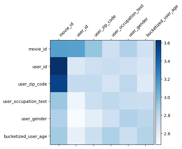
模型理解
DCN 中的權重矩陣 \(W\) 揭示了模型學習到哪些特徵交叉很重要。回想一下,在先前的玩具範例中,第 \(i\) 個和第 \(j\) 個特徵之間互動的重要性由 \(W\) 的 (\(i, j\))-th 元素捕獲。
這裡有點不同的是,特徵嵌入的大小為 32 而不是 1。因此,重要性將由 \((i, j)\)-th 區塊 \(W_{i,j}\) 表徵,其維度為 32 x 32。在以下內容中,我們視覺化每個區塊的 Frobenius 範數 [4] \(||W_{i,j}||_F\),較大的範數表示更高的重要性(假設特徵的嵌入具有相似的尺度)。
除了區塊範數之外,我們還可以視覺化整個矩陣,或每個區塊的平均值/中位數/最大值。
model = dcn_result["model"][0]
mat = model._cross_layer._dense.kernel
features = model._all_features

block_norm = np.ones([len(features), len(features)])

dim = model.embedding_dimension

# Compute the norms of the blocks.
for i in range(len(features)):
  for j in range(len(features)):
    block = mat[i * dim:(i + 1) * dim,
                j * dim:(j + 1) * dim]
    block_norm[i,j] = np.linalg.norm(block, ord="fro")

plt.figure(figsize=(9,9))
im = plt.matshow(block_norm, cmap=plt.cm.Blues)
ax = plt.gca()
divider = make_axes_locatable(plt.gca())
cax = divider.append_axes("right", size="5%", pad=0.05)
plt.colorbar(im, cax=cax)
cax.tick_params(labelsize=10)
_ = ax.set_xticklabels([""] + features, rotation=45, ha="left", fontsize=10)
_ = ax.set_yticklabels([""] + features, fontsize=10)
/tmpfs/tmp/ipykernel_40470/1244897914.py:23: UserWarning: FixedFormatter should only be used together with FixedLocator
  _ = ax.set_xticklabels([""] + features, rotation=45, ha="left", fontsize=10)
/tmpfs/tmp/ipykernel_40470/1244897914.py:24: UserWarning: FixedFormatter should only be used together with FixedLocator
  _ = ax.set_yticklabels([""] + features, fontsize=10)
<Figure size 900x900 with 0 Axes>
這就是這個 Colab 的全部內容!我們希望您喜歡學習 DCN 的一些基礎知識以及利用它的常見方法。如果您有興趣瞭解更多資訊,可以查看兩篇相關論文:DCN-v1-paper、DCN-v2-paper。
參考文獻
DCN V2:改進的深度與交叉網路以及 Web 規模學習排名系統的實務經驗.
Ruoxi Wang、Rakesh Shivanna、Derek Zhiyuan Cheng、Sagar Jain、Dong Lin、Lichan Hong、Ed Chi。(2020)
用於廣告點擊預測的深度與交叉網路.
Ruoxi Wang、Bin Fu、Gang Fu、Mingliang Wang。(AdKDD 2017)